Deep Learning – Summer 2023/24

The objective of this course is to provide a comprehensive introduction to deep neural networks, which have consistently demonstrated superior performance across diverse domains, notably in processing and generating images, text, and speech.
The course focuses both on theory spanning from the basics to the latest advances, as well as on practical implementations in Python and PyTorch (students implement and train deep neural networks performing image classification, image segmentation, object detection, part of speech tagging, lemmatization, speech recognition, reading comprehension, and image generation). Basic Python skills are required, but no previous knowledge of artificial neural networks is needed; basic machine learning understanding is advantageous.
Students work either individually or in small teams on weekly assignments, including competition tasks, where the goal is to obtain the highest performance in the class.
About
SIS code: NPFL138
Semester: summer
E-credits: 8
Examination: 3/4 C+Ex
Guarantor: Milan Straka
Timespace Coordinates
- lectures: Czech lecture is held on Monday 12:20 in S5, English lecture on Tuesday 12:20 in S4; first lecture is on Feb 19/20
- practicals: there are two parallel practicals, a Czech one on Wednesday 9:00 in S9, and an English one on Wednesday 10:40 in S9; first practicals are on Feb 21
- consultations: entirely optional consultations take place on Tuesday 15:40 in S4; first consultations are on Feb 27
All lectures and practicals will be recorded and available on this website.
Lectures
1. Introduction to Deep Learning Slides PDF Slides CZ Lecture CZ UniApprox EN Lecture EN UniApprox Questions numpy_entropy pca_first mnist_layers_activations
2. Training Neural Networks Slides PDF Slides CZ Lecture EN Lecture Questions sgd_backpropagation sgd_manual mnist_training gym_cartpole
3. Training Neural Networks II Slides PDF Slides CZ Lecture CZ Convergence EN Lecture EN Convergence Questions mnist_regularization mnist_ensemble uppercase
4. Convolutional Neural Networks Slides PDF Slides CZ Lecture EN Lecture Questions mnist_cnn torch_dataset mnist_multiple cifar_competition
5. Convolutional Neural Networks II Slides PDF Slides CZ Lecture EN Lecture EN Transposed Convolution Questions cnn_manual cags_classification cags_segmentation
6. Object Detection Slides PDF Slides CZ Lecture EN Lecture Questions bboxes_utils svhn_competition
7. Easter Monday 3d_recognition
8. Recurrent Neural Networks Slides PDF Slides CZ Lecture EN Lecture Questions sequence_classification tagger_we tagger_cle tagger_competition
9. Structured Prediction, CTC, Word2Vec Slides PDF Slides CZ Lecture EN Lecture Questions tensorboard_projector tagger_ner ctc_loss speech_recognition
10. Seq2seq, NMT, Transformer Slides PDF Slides CZ Lecture EN Lecture Questions lemmatizer_noattn lemmatizer_attn lemmatizer_competition
11. Transformer, BERT, ViT Slides PDF Slides CZ Lecture EN Lecture Questions tagger_transformer sentiment_analysis reading_comprehension
12. Deep Reinforcement Learning, VAE Slides PDF Slides CZ Lecture EN Lecture Questions homr_competition reinforce reinforce_baseline reinforce_pixels vae
13. Generative Adversarial Networks, Diffusion Models Slides PDF Slides CZ Lecture CZ Stable Diffusion, Score-based Models EN Lecture Questions gan dcgan ddim ddim_attention ddim_conditional
14. Speech Synthesis, External Memory, Meta-Learning Slides PDF Slides CZ Lecture EN Lecture Questions learning_to_learn
License
Unless otherwise stated, teaching materials for this course are available under CC BY-SA 4.0.
The lecture content, including references to study materials. The main study material is the Deep Learning Book by Ian Goodfellow, Yoshua Bengio and Aaron Courville, (referred to as DLB).
References to study materials cover all theory required at the exam, and sometimes even more – the references in italics cover topics not required for the exam.
1. Introduction to Deep Learning
Feb 19 Slides PDF Slides CZ Lecture CZ UniApprox EN Lecture EN UniApprox Questions numpy_entropy pca_first mnist_layers_activations
- Random variables, probability distributions, expectation, variance, Bernoulli distribution, Categorical distribution [Sections 3.2, 3.3, 3.8, 3.9.1 and 3.9.2 of DLB]
- Self-information, entropy, cross-entropy, KL-divergence [Section 3.13 of DBL]
- Gaussian distribution [Section 3.9.3 of DLB]
- Machine Learning Basics [Section 5.1-5.1.3 of DLB]
- History of Deep Learning [Section 1.2 of DLB]
- Linear regression [Section 5.1.4 of DLB]
- Challenges Motivating Deep Learning [Section 5.11 of DLB]
- Neural network basics
- Neural networks as graphs [Chapter 6 before Section 6.1 of DLB]
- Output activation functions [Section 6.2.2 of DLB, excluding Section 6.2.2.4]
- Hidden activation functions [Section 6.3 of DLB, excluding Section 6.3.3]
- Basic network architectures [Section 6.4 of DLB, excluding Section 6.4.2]
- Universal approximation theorem
2. Training Neural Networks
Feb 26 Slides PDF Slides CZ Lecture EN Lecture Questions sgd_backpropagation sgd_manual mnist_training gym_cartpole
- Capacity, overfitting, underfitting, regularization [Section 5.2 of DLB]
- Hyperparameters and validation sets [Section 5.3 of DLB]
- Maximum Likelihood Estimation [Section 5.5 of DLB]
- Neural network training
- Gradient Descent and Stochastic Gradient Descent [Sections 4.3 and 5.9 of DLB]
- Backpropagation algorithm [Section 6.5 to 6.5.3 of DLB, especially Algorithms 6.1 and 6.2; note that Algorithms 6.5 and 6.6 are used in practice]
- SGD algorithm [Section 8.3.1 and Algorithm 8.1 of DLB]
- SGD with Momentum algorithm [Section 8.3.2 and Algorithm 8.2 of DLB]
- SGD with Nestorov Momentum algorithm [Section 8.3.3 and Algorithm 8.3 of DLB]
- Optimization algorithms with adaptive gradients
- AdaGrad algorithm [Section 8.5.1 and Algorithm 8.4 of DLB]
- RMSProp algorithm [Section 8.5.2 and Algorithm 8.5 of DLB]
- Adam algorithm [Section 8.5.3 and Algorithm 8.7 of DLB]
3. Training Neural Networks II
Mar 4 Slides PDF Slides CZ Lecture CZ Convergence EN Lecture EN Convergence Questions mnist_regularization mnist_ensemble uppercase
- Softmax with NLL (negative log likelihood) as a loss function [Section 6.2.2.3 of DLB, notably equation (6.30); plus slides 10-12]
- Regularization [Chapter 7 until Section 7.1 of DLB]
- Early stopping [Section 7.8 of DLB, without the How early stopping acts as a regularizer part]
- L2 and L1 regularization [Sections 7.1 and 5.6.1 of DLB; plus slides 17-18]
- Dataset augmentation [Section 7.4 of DLB]
- Ensembling [Section 7.11 of DLB]
- Dropout [Section 7.12 of DLB]
- Label smoothing [Section 7.5.1 of DLB]
- Saturating non-linearities [Section 6.3.2 and second half of Section 6.2.2.2 of DLB]
- Parameter initialization strategies [Section 8.4 of DLB]
- Gradient clipping [Section 10.11.1 of DLB]
4. Convolutional Neural Networks
Mar 11 Slides PDF Slides CZ Lecture EN Lecture Questions mnist_cnn torch_dataset mnist_multiple cifar_competition
- Introduction to convolutional networks [Chapter 9 and Sections 9.1-9.3 of DLB]
- Convolution as operation on 4D tensors [Section 9.5 of DLB, notably Equations (9.7) and (9.8)]
- Max pooling and average pooling [Section 9.3 of DLB]
- Stride and Padding schemes [Section 9.5 of DLB]
- AlexNet [ImageNet Classification with Deep Convolutional Neural Networks]
- VGG [Very Deep Convolutional Networks for Large-Scale Image Recognition]
- GoogLeNet (aka Inception) [Going Deeper with Convolutions]
- Batch normalization [Section 8.7.1 of DLB, optionally the paper Batch Normalization: Accelerating Deep Network Training by Reducing Internal Covariate Shift]
- Inception v2 and v3 [Rethinking the Inception Architecture for Computer Vision]
- ResNet [Deep Residual Learning for Image Recognition]
5. Convolutional Neural Networks II
Mar 18 Slides PDF Slides CZ Lecture EN Lecture EN Transposed Convolution Questions cnn_manual cags_classification cags_segmentation
- Residual CNN Networks
- ResNet [Deep Residual Learning for Image Recognition]
- WideNet [Wide Residual Network]
- DenseNet [Densely Connected Convolutional Networks]
- PyramidNet [Deep Pyramidal Residual Networks]
- ResNeXt [Aggregated Residual Transformations for Deep Neural Networks]
- Regularizing CNN Networks
- SENet [Squeeze-and-Excitation Networks]
- EfficientNet [EfficientNet: Rethinking Model Scaling for Convolutional Neural Networks]
- EfficientNetV2 [EfficientNetV2: Smaller Models and Faster Training]
- Transposed convolution
- U-Net [U-Net: Convolutional Networks for Biomedical Image Segmentation]
6. Object Detection
Mar 25 Slides PDF Slides CZ Lecture EN Lecture Questions bboxes_utils svhn_competition
- R-CNN [R-CNN]
- Fast R-CNN [Fast R-CNN]
- Proposing RoIs using Faster R-CNN [Faster R-CNN: Towards Real-Time Object Detection with Region Proposal Networks]
- Mask R-CNN [Mask R-CNN]
- Feature Pyramid Networks [Feature Pyramid Networks for Object Detection]
- Focal Loss, RetinaNet [Focal Loss for Dense Object Detection]
- EfficientDet [EfficientDet: Scalable and Efficient Object Detection]
- Group Normalization [Group Normalization]
7. Easter Monday
Apr 01 3d_recognition
8. Recurrent Neural Networks
Apr 8 Slides PDF Slides CZ Lecture EN Lecture Questions sequence_classification tagger_we tagger_cle tagger_competition
- Sequence modelling using Recurrent Neural Networks (RNN) [Chapter 10 until Section 10.2.1 (excluding) of DLB]
- The challenge of long-term dependencies [Section 10.7 of DLB]
- Long Short-Term Memory (LSTM) [Section 10.10.1 of DLB, Sepp Hochreiter, Jürgen Schmidhuber (1997): Long short-term memory, Felix A. Gers, Jürgen Schmidhuber, Fred Cummins (2000): Learning to Forget: Continual Prediction with LSTM]
- Gated Recurrent Unit (GRU) [Section 10.10.2 of DLB, Kyunghyun Cho, Bart van Merrienboer, Caglar Gulcehre, Dzmitry Bahdanau, Fethi Bougares, Holger Schwenk, Yoshua Bengio: Learning Phrase Representations using RNN Encoder-Decoder for Statistical Machine Translation]
- Highway Networks [Training Very Deep Networks]
- RNN Regularization
- Variational Dropout [A Theoretically Grounded Application of Dropout in Recurrent Neural Networks]
- Layer Normalization [Layer Normalization]
- Bidirectional RNN [Section 10.3 of DLB]
- Word Embeddings [Section 14.2.4 of DLB]
- Character-level embeddings using Recurrent neural networks [C2W model from Finding Function in Form: Compositional Character Models for Open Vocabulary Word Representation]
- Character-level embeddings using Convolutional neural networks [CharCNN from Character-Aware Neural Language Models]
9. Structured Prediction, CTC, Word2Vec
Apr 15 Slides PDF Slides CZ Lecture EN Lecture Questions tensorboard_projector tagger_ner ctc_loss speech_recognition
- Structured prediction
- Connectionist Temporal Classification (CTC) loss [Connectionist Temporal Classification: Labelling Unsegmented Sequence Data with Recurrent Neural Networks]
Word2vecword embeddings, notably the CBOW and Skip-gram architectures [Efficient Estimation of Word Representations in Vector Space]- Hierarchical softmax [Section 12.4.3.2 of DLB or Distributed Representations of Words and Phrases and their Compositionality]
- Negative sampling Distributed Representations of Words and Phrases and their Compositionality]
- Character-level embeddings using character n-grams [Described simultaneously in several papers as Charagram (Charagram: Embedding Words and Sentences via Character n-grams), Subword Information (Enriching Word Vectors with Subword Information or SubGram (SubGram: Extending Skip-Gram Word Representation with Substrings)]
- ELMO [Matthew E. Peters, Mark Neumann, Mohit Iyyer, Matt Gardner, Christopher Clark, Kenton Lee, Luke Zettlemoyer: Deep contextualized word representations]
10. Seq2seq, NMT, Transformer
Apr 22 Slides PDF Slides CZ Lecture EN Lecture Questions lemmatizer_noattn lemmatizer_attn lemmatizer_competition
- Neural Machine Translation using Encoder-Decoder or Sequence-to-Sequence architecture [Section 12.5.4 of DLB, Ilya Sutskever, Oriol Vinyals, Quoc V. Le: Sequence to Sequence Learning with Neural Networks and Kyunghyun Cho et al.: Learning Phrase Representations using RNN Encoder-Decoder for Statistical Machine Translation]
- Using Attention mechanism in Neural Machine Translation [Section 12.4.5.1 of DLB, Dzmitry Bahdanau, Kyunghyun Cho, Yoshua Bengio: Neural Machine Translation by Jointly Learning to Align and Translate]
- Translating Subword Units [Rico Sennrich, Barry Haddow, Alexandra Birch: Neural Machine Translation of Rare Words with Subword Units]
- Google NMT [Yonghui Wu et al.: Google's Neural Machine Translation System: Bridging the Gap between Human and Machine Translation]
- Transformer architecture [Attention Is All You Need]
11. Transformer, BERT, ViT
Apr 29 Slides PDF Slides CZ Lecture EN Lecture Questions tagger_transformer sentiment_analysis reading_comprehension
- Transformer architecture [Attention Is All You Need]
- BERT [BERT: Pre-training of Deep Bidirectional Transformers for Language Understanding]
- RoBERTa [RoBERTa: A Robustly Optimized BERT Pretraining Approach]
- ViT [An Image is Worth 16x16 Words: Transformers for Image Recognition at Scale]
- MAE [Masked Autoencoders Are Scalable Vision Learners]
- DETR [End-to-End Object Detection with Transformers]
12. Deep Reinforcement Learning, VAE
May 6 Slides PDF Slides CZ Lecture EN Lecture Questions homr_competition reinforce reinforce_baseline reinforce_pixels vae
Study material for Reinforcement Learning is the Reinforcement Learning: An Introduction; second edition by Richard S. Sutton and Andrew G. Barto (reffered to as RLB), available online.
- Multi-armed bandits [Sections 2-2.4 of RLB]
- Markov Decision Process [Sections 3-3.3 of RLB]
- Policies and Value Functions [Sections 3.5 of RLB]
- Policy Gradient Methods [Sections 13-13.1 of RLB]
- Policy Gradient Theorem [Section 13.2 of RLB]
- REINFORCE algorithm [Section 13.3 of RLB]
- REINFORCE with baseline algorithm [Section 13.4 of RLB]
- Autoencoders (undercomplete, sparse, denoising) [Chapter 14, Sections 14-14.2.3 of DLB]
- Deep Generative Models using Differentiable Generator Nets [Section 20.10.2 of DLB]
- Variational Autoencoders [Section 20.10.3 plus Reparametrization trick from Section 20.9 (but not Section 20.9.1) of DLB, Auto-Encoding Variational Bayes]
13. Generative Adversarial Networks, Diffusion Models
May 13 Slides PDF Slides CZ Lecture CZ Stable Diffusion, Score-based Models EN Lecture Questions gan dcgan ddim ddim_attention ddim_conditional
- Generative Adversarial Networks
- GAN [Section 20.10.4 of DLB, Generative Adversarial Networks]
- CGAN [Conditional Generative Adversarial Nets]
- DCGAN [Unsupervised Representation Learning with Deep Convolutional Generative Adversarial Networks]
- Diffusion Models
14. Speech Synthesis, External Memory, Meta-Learning
May 20 Slides PDF Slides CZ Lecture EN Lecture Questions learning_to_learn
- WaveNet [WaveNet: A Generative Model for Raw Audio]
- Parallel WaveNet [Parallel WaveNet: Fast High-Fidelity Speech Synthesis]
- Full speech synthesis pipeline Tacotron 2 [Natural TTS Synthesis by Conditioning WaveNet on Mel Spectrogram Predictions]
- Neural Turing Machine [Neural Turing Machines]
- Memory Augmented Neural Networks [One-shot learning with Memory-Augmented Neural Networks]
- Differenciable Neural Computer [Hybrid computing using a neural network with dynamic external memory]
- Token Turing Machine [Token Turing Machines]
Requirements
To pass the practicals, you need to obtain at least 80 points, excluding the bonus points. Note that all surplus points (both bonus and non-bonus) will be transfered to the exam. In total, assignments for at least 120 points (not including the bonus points) will be available, and if you solve all the assignments (any non-zero amount of points counts as solved), you automatically pass the exam with grade 1.
Environment
The tasks are evaluated automatically using the ReCodEx Code Examiner.
The evaluation is performed using Python 3.11, Keras 3.0.5, PyTorch 2.2.0, HF Transformers 4.37.2, and Gymnasium 1.0.0a. You should install the exact version of these packages yourselves.
Teamwork
Solving assignments in teams (of size at most 3) is encouraged, but everyone has to participate (it is forbidden not to work on an assignment and then submit a solution created by other team members). All members of the team must submit in ReCodEx individually, but can have exactly the same sources/models/results. Each such solution must explicitly list all members of the team to allow plagiarism detection using this template.
No Cheating
Cheating is strictly prohibited and any student found cheating will be punished. The punishment can involve failing the whole course, or, in grave cases, being expelled from the faculty. While discussing assignments with any classmate is fine, each team must complete the assignments themselves, without using code they did not write (unless explicitly allowed). Of course, inside a team you are allowed to share code and submit identical solutions. Note that all students involved in cheating will be punished, so if you share your source code with a friend, both you and your friend will be punished. That also means that you should never publish your solutions.
numpy_entropy
Deadline: Mar 05, 22:00 3 points
The goal of this exercise is to familiarize with Python, NumPy and ReCodEx submission system. Start with the numpy_entropy.py.
Load a file specified in args.data_path, whose lines consist of data points of our
dataset, and load a file specified in args.model_path, which describes a model probability distribution,
with each line being a tab-separated pair of (data point, probability).
Then compute the following quantities using NumPy, and print them each on
a separate line rounded on two decimal places (or inf for positive infinity,
which happens when an element of data distribution has zero probability
under the model distribution):
- entropy H(data distribution)
- cross-entropy H(data distribution, model distribution)
- KL-divergence DKL(data distribution, model distribution)
Use natural logarithms to compute the entropies and the divergence.
python3 numpy_entropy.py --data_pathnumpy_entropy_data_1.txt--model_pathnumpy_entropy_model_1.txt
Entropy: 0.96 nats
Crossentropy: 0.99 nats
KL divergence: 0.03 nats
python3 numpy_entropy.py --data_pathnumpy_entropy_data_2.txt--model_pathnumpy_entropy_model_2.txt
Entropy: 0.96 nats
Crossentropy: inf nats
KL divergence: inf nats
- The last three tests use data available only in ReCodEx. They are analogous to the numpy_entropy_data_3.txt numpy_entropy_model_3.txt and numpy_entropy_data_4.txt numpy_entropy_model_4.txt, but are generated with different random seeds.
Note that your results may be slightly different, depending on your CPU type and whether you use a GPU.
python3 numpy_entropy.py --data_pathnumpy_entropy_data_1.txt--model_pathnumpy_entropy_model_1.txt
Entropy: 0.96 nats
Crossentropy: 0.99 nats
KL divergence: 0.03 nats
python3 numpy_entropy.py --data_pathnumpy_entropy_data_2.txt--model_pathnumpy_entropy_model_2.txt
Entropy: 0.96 nats
Crossentropy: inf nats
KL divergence: inf nats
python3 numpy_entropy.py --data_pathnumpy_entropy_data_3.txt--model_pathnumpy_entropy_model_3.txt
Entropy: 4.15 nats
Crossentropy: 4.23 nats
KL divergence: 0.08 nats
python3 numpy_entropy.py --data_pathnumpy_entropy_data_4.txt--model_pathnumpy_entropy_model_4.txt
Entropy: 4.99 nats
Crossentropy: 5.03 nats
KL divergence: 0.04 nats
pca_first
Deadline: Mar 05, 22:00 2 points
The goal of this exercise is to familiarize with PyTorch torch.Tensors,
shapes and basic tensor manipulation methods. Start with the
pca_first.py
(and you will also need the mnist.py
module).
Alternatively, you can instead use the
pca_first.keras.py
template, which uses backend-agnostic keras.ops operations instead of PyTorch
operations – both templates can be used to solve the assignment.
In this assignment, you should compute the covariance matrix of several examples from the MNIST dataset, then compute the first principal component, and quantify the explained variance of it. It is fine if you are not familiar with terms like covariance matrix or principal component – the template contains a detailed description of what you have to do.
Finally, you might want to read the Introduction to PyTorch Tensors.
Note that your results may be slightly different, depending on your CPU type and whether you use a GPU.
python3 pca_first.py --examples=1024 --iterations=64
Total variance: 53.12
Explained variance: 9.64%
python3 pca_first.py --examples=8192 --iterations=128
Total variance: 53.05
Explained variance: 9.89%
python3 pca_first.py --examples=55000 --iterations=1024
Total variance: 52.74
Explained variance: 9.71%
mnist_layers_activations
Deadline: Mar 05, 22:00 2 points
Before solving the assignment, start by playing with
example_keras_tensorboard.py,
in order to familiarize with Keras and TensorBoard.
Run it, and when it finishes, run TensorBoard using tensorboard --logdir logs.
Then open http://localhost:6006 in a browser and explore the active tabs.
Your goal is to modify the mnist_layers_activations.py template such that a user-specified neural network is constructed:
- A number of hidden layers (including zero) can be specified on the command line
using parameter
hidden_layers. - Activation function of these hidden layers can be also specified as a command
line parameter
activation, with supported values ofnone,relu,tanhandsigmoid.
Note that your results may be slightly different, depending on your CPU type and whether you use a GPU.
python3 mnist_layers_activations.py --epochs=1 --hidden_layers=0 --activation=none
accuracy: 0.7801 - loss: 0.8405 - val_accuracy: 0.9300 - val_loss: 0.2716
python3 mnist_layers_activations.py --epochs=1 --hidden_layers=1 --activation=none
accuracy: 0.8483 - loss: 0.5230 - val_accuracy: 0.9352 - val_loss: 0.2422
python3 mnist_layers_activations.py --epochs=1 --hidden_layers=1 --activation=relu
accuracy: 0.8503 - loss: 0.5286 - val_accuracy: 0.9604 - val_loss: 0.1432
python3 mnist_layers_activations.py --epochs=1 --hidden_layers=1 --activation=tanh
accuracy: 0.8529 - loss: 0.5183 - val_accuracy: 0.9564 - val_loss: 0.1632
python3 mnist_layers_activations.py --epochs=1 --hidden_layers=1 --activation=sigmoid
accuracy: 0.7851 - loss: 0.8650 - val_accuracy: 0.9414 - val_loss: 0.2196
python3 mnist_layers_activations.py --epochs=1 --hidden_layers=3 --activation=relu
accuracy: 0.8497 - loss: 0.5011 - val_accuracy: 0.9664 - val_loss: 0.1225
Note that your results may be slightly different, depending on your CPU type and whether you use a GPU.
python3 mnist_layers_activations.py --hidden_layers=0 --activation=none
Epoch  1/10 accuracy: 0.7801 - loss: 0.8405 - val_accuracy: 0.9300 - val_loss: 0.2716
Epoch  5/10 accuracy: 0.9222 - loss: 0.2792 - val_accuracy: 0.9406 - val_loss: 0.2203
Epoch 10/10 accuracy: 0.9304 - loss: 0.2515 - val_accuracy: 0.9432 - val_loss: 0.2159
python3 mnist_layers_activations.py --hidden_layers=1 --activation=none
Epoch  1/10 accuracy: 0.8483 - loss: 0.5230 - val_accuracy: 0.9352 - val_loss: 0.2422
Epoch  5/10 accuracy: 0.9236 - loss: 0.2758 - val_accuracy: 0.9360 - val_loss: 0.2325
Epoch 10/10 accuracy: 0.9298 - loss: 0.2517 - val_accuracy: 0.9354 - val_loss: 0.2439
python3 mnist_layers_activations.py --hidden_layers=1 --activation=relu
Epoch  1/10 accuracy: 0.8503 - loss: 0.5286 - val_accuracy: 0.9604 - val_loss: 0.1432
Epoch  5/10 accuracy: 0.9824 - loss: 0.0613 - val_accuracy: 0.9808 - val_loss: 0.0740
Epoch 10/10 accuracy: 0.9948 - loss: 0.0202 - val_accuracy: 0.9788 - val_loss: 0.0821
python3 mnist_layers_activations.py --hidden_layers=1 --activation=tanh
Epoch  1/10 accuracy: 0.8529 - loss: 0.5183 - val_accuracy: 0.9564 - val_loss: 0.1632
Epoch  5/10 accuracy: 0.9800 - loss: 0.0728 - val_accuracy: 0.9740 - val_loss: 0.0853
Epoch 10/10 accuracy: 0.9948 - loss: 0.0244 - val_accuracy: 0.9782 - val_loss: 0.0772
python3 mnist_layers_activations.py --hidden_layers=1 --activation=sigmoid
Epoch  1/10 accuracy: 0.7851 - loss: 0.8650 - val_accuracy: 0.9414 - val_loss: 0.2196
Epoch  5/10 accuracy: 0.9647 - loss: 0.1270 - val_accuracy: 0.9704 - val_loss: 0.1079
Epoch 10/10 accuracy: 0.9852 - loss: 0.0583 - val_accuracy: 0.9756 - val_loss: 0.0837
python3 mnist_layers_activations.py --hidden_layers=3 --activation=relu
Epoch  1/10 accuracy: 0.8497 - loss: 0.5011 - val_accuracy: 0.9664 - val_loss: 0.1225
Epoch  5/10 accuracy: 0.9862 - loss: 0.0438 - val_accuracy: 0.9734 - val_loss: 0.1026
Epoch 10/10 accuracy: 0.9932 - loss: 0.0202 - val_accuracy: 0.9818 - val_loss: 0.0865
python3 mnist_layers_activations.py --hidden_layers=10 --activation=relu
Epoch  1/10 accuracy: 0.7710 - loss: 0.6793 - val_accuracy: 0.9570 - val_loss: 0.1479
Epoch  5/10 accuracy: 0.9780 - loss: 0.0783 - val_accuracy: 0.9786 - val_loss: 0.0808
Epoch 10/10 accuracy: 0.9869 - loss: 0.0481 - val_accuracy: 0.9724 - val_loss: 0.1163
python3 mnist_layers_activations.py --hidden_layers=10 --activation=sigmoid
Epoch  1/10 accuracy: 0.1072 - loss: 2.3068 - val_accuracy: 0.1784 - val_loss: 2.1247
Epoch  5/10 accuracy: 0.8825 - loss: 0.4776 - val_accuracy: 0.9164 - val_loss: 0.3686
Epoch 10/10 accuracy: 0.9294 - loss: 0.2994 - val_accuracy: 0.9386 - val_loss: 0.2671
sgd_backpropagation
Deadline: Mar 12, 22:00 3 points
In this exercise you will learn how to compute gradients using the so-called automatic differentiation, which allows to automatically run backpropagation algorithm for a given computation. You can read the Automatic Differentiation with torch.autograd tutorial if interested. After computing the gradient, you should then perform training by running manually implemented minibatch stochastic gradient descent.
Starting with the sgd_backpropagation.py template, you should:
- implement a neural network with a single tanh hidden layer and categorical output layer;
- compute the crossentropy loss;
- use
.backward()to automatically compute the gradient of the loss with respect to all variables; - perform the SGD update.
Note that your results may be slightly different, depending on your CPU type and whether you use a GPU.
python3 sgd_backpropagation.py --epochs=2 --batch_size=64 --hidden_layer=20 --learning_rate=0.1
Dev accuracy after epoch 1 is 93.30
Dev accuracy after epoch 2 is 94.38
Test accuracy after epoch 2 is 93.15
python3 sgd_backpropagation.py --epochs=2 --batch_size=100 --hidden_layer=32 --learning_rate=0.2
Dev accuracy after epoch 1 is 93.64
Dev accuracy after epoch 2 is 94.80
Test accuracy after epoch 2 is 93.54
Note that your results may be slightly different, depending on your CPU type and whether you use a GPU.
python3 sgd_backpropagation.py --batch_size=64 --hidden_layer=20 --learning_rate=0.1
Dev accuracy after epoch 1 is 93.30
Dev accuracy after epoch 2 is 94.38
Dev accuracy after epoch 3 is 95.16
Dev accuracy after epoch 4 is 95.50
Dev accuracy after epoch 5 is 95.96
Dev accuracy after epoch 6 is 96.04
Dev accuracy after epoch 7 is 95.82
Dev accuracy after epoch 8 is 95.92
Dev accuracy after epoch 9 is 95.96
Dev accuracy after epoch 10 is 96.16
Test accuracy after epoch 10 is 95.26
python3 sgd_backpropagation.py --batch_size=100 --hidden_layer=32 --learning_rate=0.2
Dev accuracy after epoch 1 is 93.64
Dev accuracy after epoch 2 is 94.80
Dev accuracy after epoch 3 is 95.56
Dev accuracy after epoch 4 is 95.98
Dev accuracy after epoch 5 is 96.24
Dev accuracy after epoch 6 is 96.74
Dev accuracy after epoch 7 is 96.52
Dev accuracy after epoch 8 is 96.54
Dev accuracy after epoch 9 is 97.04
Dev accuracy after epoch 10 is 97.02
Test accuracy after epoch 10 is 96.16
sgd_manual 

Deadline: Mar 12, 22:00 2 points
The goal in this exercise is to extend your solution to the sgd_backpropagation assignment by manually computing the gradient.
While in this assignment we compute the gradient manually, we will nearly always use the automatic differentiation. Therefore, the assignment is more of a mathematical exercise than a real-world application. Furthermore, we will compute the derivatives together on the Mar 06 practicals.
Start with the sgd_manual.py template, which is based on sgd_backpropagation.py one.
Note that ReCodEx disables the PyTorch automatic differentiation during evaluation.
Note that your results may be slightly different, depending on your CPU type and whether you use a GPU.
python3 sgd_manual.py --epochs=2 --batch_size=64 --hidden_layer=20 --learning_rate=0.1
Dev accuracy after epoch 1 is 93.30
Dev accuracy after epoch 2 is 94.38
Test accuracy after epoch 2 is 93.15
python3 sgd_manual.py --epochs=2 --batch_size=100 --hidden_layer=32 --learning_rate=0.2
Dev accuracy after epoch 1 is 93.64
Dev accuracy after epoch 2 is 94.80
Test accuracy after epoch 2 is 93.54
Note that your results may be slightly different, depending on your CPU type and whether you use a GPU.
python3 sgd_manual.py --batch_size=64 --hidden_layer=20 --learning_rate=0.1
Dev accuracy after epoch 1 is 93.30
Dev accuracy after epoch 2 is 94.38
Dev accuracy after epoch 3 is 95.16
Dev accuracy after epoch 4 is 95.50
Dev accuracy after epoch 5 is 95.96
Dev accuracy after epoch 6 is 96.04
Dev accuracy after epoch 7 is 95.82
Dev accuracy after epoch 8 is 95.92
Dev accuracy after epoch 9 is 95.96
Dev accuracy after epoch 10 is 96.16
Test accuracy after epoch 10 is 95.26
python3 sgd_manual.py --batch_size=100 --hidden_layer=32 --learning_rate=0.2
Dev accuracy after epoch 1 is 93.64
Dev accuracy after epoch 2 is 94.80
Dev accuracy after epoch 3 is 95.56
Dev accuracy after epoch 4 is 95.98
Dev accuracy after epoch 5 is 96.24
Dev accuracy after epoch 6 is 96.74
Dev accuracy after epoch 7 is 96.52
Dev accuracy after epoch 8 is 96.54
Dev accuracy after epoch 9 is 97.04
Dev accuracy after epoch 10 is 97.02
Test accuracy after epoch 10 is 96.16
mnist_training
Deadline: Mar 12, 22:00 2 points
This exercise should teach you using different optimizers, learning rates, and learning rate decays. Your goal is to modify the mnist_training.py template and implement the following:
- Using specified optimizer (either
SGDorAdam). - Optionally using momentum for the
SGDoptimizer. - Using specified learning rate for the optimizer.
- Optionally use a given learning rate schedule. The schedule can be either
linear,exponential, orcosine. If a schedule is specified, you also get a final learning rate, and the learning rate should be gradually decresed during training to reach the final learning rate just after the training (i.e., the first update after the training would use exactly the final learning rate).
Note that your results may be slightly different, depending on your CPU type and whether you use a GPU.
python3 mnist_training.py --epochs=1 --optimizer=SGD --learning_rate=0.01
accuracy: 0.6537 - loss: 1.2786 - val_accuracy: 0.9098 - val_loss: 0.3743
python3 mnist_training.py --epochs=1 --optimizer=SGD --learning_rate=0.01 --momentum=0.9
accuracy: 0.8221 - loss: 0.6138 - val_accuracy: 0.9492 - val_loss: 0.1873
python3 mnist_training.py --epochs=1 --optimizer=SGD --learning_rate=0.1
accuracy: 0.8400 - loss: 0.5742 - val_accuracy: 0.9528 - val_loss: 0.1800
python3 mnist_training.py --epochs=1 --optimizer=Adam --learning_rate=0.001
accuracy: 0.8548 - loss: 0.5121 - val_accuracy: 0.9640 - val_loss: 0.1327
python3 mnist_training.py --epochs=1 --optimizer=Adam --learning_rate=0.01
accuracy: 0.8858 - loss: 0.3598 - val_accuracy: 0.9564 - val_loss: 0.1393
python3 mnist_training.py --epochs=2 --optimizer=Adam --learning_rate=0.01 --decay=linear --learning_rate_final=0.0001
Epoch 1/2 accuracy: 0.8889 - loss: 0.3520 - val_accuracy: 0.9682 - val_loss: 0.1107
Epoch 2/2 accuracy: 0.9715 - loss: 0.0956 - val_accuracy: 0.9792 - val_loss: 0.0688
Next learning rate to be used: 0.0001
python3 mnist_training.py --epochs=2 --optimizer=Adam --learning_rate=0.01 --decay=exponential --learning_rate_final=0.001
Epoch 1/2 accuracy: 0.8912 - loss: 0.3447 - val_accuracy: 0.9702 - val_loss: 0.0997
Epoch 2/2 accuracy: 0.9746 - loss: 0.0824 - val_accuracy: 0.9778 - val_loss: 0.0776
Next learning rate to be used: 0.001
python3 mnist_training.py --epochs=2 --optimizer=Adam --learning_rate=0.01 --decay=cosine --learning_rate_final=0.0001
Epoch 1/2 accuracy: 0.8875 - loss: 0.3548 - val_accuracy: 0.9726 - val_loss: 0.0976
Epoch 2/2 accuracy: 0.9742 - loss: 0.0851 - val_accuracy: 0.9764 - val_loss: 0.0740
Next learning rate to be used: 0.0001
Note that your results may be slightly different, depending on your CPU type and whether you use a GPU.
python3 mnist_training.py --optimizer=SGD --learning_rate=0.01
Epoch  1/10 accuracy: 0.6537 - loss: 1.2786 - val_accuracy: 0.9098 - val_loss: 0.3743
Epoch  2/10 accuracy: 0.8848 - loss: 0.4316 - val_accuracy: 0.9222 - val_loss: 0.2895
Epoch  3/10 accuracy: 0.9057 - loss: 0.3450 - val_accuracy: 0.9308 - val_loss: 0.2539
Epoch  4/10 accuracy: 0.9118 - loss: 0.3131 - val_accuracy: 0.9372 - val_loss: 0.2368
Epoch  5/10 accuracy: 0.9188 - loss: 0.2924 - val_accuracy: 0.9406 - val_loss: 0.2202
Epoch  6/10 accuracy: 0.9235 - loss: 0.2750 - val_accuracy: 0.9426 - val_loss: 0.2076
Epoch  7/10 accuracy: 0.9291 - loss: 0.2572 - val_accuracy: 0.9464 - val_loss: 0.1997
Epoch  8/10 accuracy: 0.9304 - loss: 0.2456 - val_accuracy: 0.9494 - val_loss: 0.1909
Epoch  9/10 accuracy: 0.9339 - loss: 0.2340 - val_accuracy: 0.9536 - val_loss: 0.1813
Epoch 10/10 accuracy: 0.9377 - loss: 0.2199 - val_accuracy: 0.9534 - val_loss: 0.1756
python3 mnist_training.py --optimizer=SGD --learning_rate=0.01 --momentum=0.9
Epoch  1/10 accuracy: 0.8221 - loss: 0.6138 - val_accuracy: 0.9492 - val_loss: 0.1873
Epoch  2/10 accuracy: 0.9370 - loss: 0.2173 - val_accuracy: 0.9646 - val_loss: 0.1385
Epoch  3/10 accuracy: 0.9599 - loss: 0.1453 - val_accuracy: 0.9716 - val_loss: 0.1076
Epoch  4/10 accuracy: 0.9673 - loss: 0.1127 - val_accuracy: 0.9746 - val_loss: 0.0961
Epoch  5/10 accuracy: 0.9740 - loss: 0.0933 - val_accuracy: 0.9774 - val_loss: 0.0875
Epoch  6/10 accuracy: 0.9778 - loss: 0.0811 - val_accuracy: 0.9746 - val_loss: 0.0856
Epoch  7/10 accuracy: 0.9821 - loss: 0.0680 - val_accuracy: 0.9774 - val_loss: 0.0803
Epoch  8/10 accuracy: 0.9825 - loss: 0.0632 - val_accuracy: 0.9776 - val_loss: 0.0780
Epoch  9/10 accuracy: 0.9849 - loss: 0.0552 - val_accuracy: 0.9804 - val_loss: 0.0725
Epoch 10/10 accuracy: 0.9877 - loss: 0.0463 - val_accuracy: 0.9780 - val_loss: 0.0735
python3 mnist_training.py --optimizer=SGD --learning_rate=0.1
Epoch  1/10 accuracy: 0.8400 - loss: 0.5742 - val_accuracy: 0.9528 - val_loss: 0.1800
Epoch  2/10 accuracy: 0.9389 - loss: 0.2123 - val_accuracy: 0.9670 - val_loss: 0.1335
Epoch  3/10 accuracy: 0.9602 - loss: 0.1431 - val_accuracy: 0.9728 - val_loss: 0.1052
Epoch  4/10 accuracy: 0.9685 - loss: 0.1115 - val_accuracy: 0.9770 - val_loss: 0.0946
Epoch  5/10 accuracy: 0.9747 - loss: 0.0927 - val_accuracy: 0.9754 - val_loss: 0.0878
Epoch  6/10 accuracy: 0.9775 - loss: 0.0798 - val_accuracy: 0.9754 - val_loss: 0.0852
Epoch  7/10 accuracy: 0.9813 - loss: 0.0680 - val_accuracy: 0.9780 - val_loss: 0.0797
Epoch  8/10 accuracy: 0.9828 - loss: 0.0621 - val_accuracy: 0.9796 - val_loss: 0.0757
Epoch  9/10 accuracy: 0.9847 - loss: 0.0550 - val_accuracy: 0.9804 - val_loss: 0.0731
Epoch 10/10 accuracy: 0.9875 - loss: 0.0464 - val_accuracy: 0.9782 - val_loss: 0.0731
python3 mnist_training.py --optimizer=Adam --learning_rate=0.001
Epoch  1/10 accuracy: 0.8548 - loss: 0.5121 - val_accuracy: 0.9640 - val_loss: 0.1327
Epoch  2/10 accuracy: 0.9552 - loss: 0.1505 - val_accuracy: 0.9706 - val_loss: 0.1118
Epoch  3/10 accuracy: 0.9744 - loss: 0.0900 - val_accuracy: 0.9770 - val_loss: 0.0833
Epoch  4/10 accuracy: 0.9808 - loss: 0.0658 - val_accuracy: 0.9778 - val_loss: 0.0786
Epoch  5/10 accuracy: 0.9836 - loss: 0.0533 - val_accuracy: 0.9804 - val_loss: 0.0735
Epoch  6/10 accuracy: 0.9890 - loss: 0.0403 - val_accuracy: 0.9782 - val_loss: 0.0772
Epoch  7/10 accuracy: 0.9911 - loss: 0.0311 - val_accuracy: 0.9792 - val_loss: 0.0756
Epoch  8/10 accuracy: 0.9922 - loss: 0.0257 - val_accuracy: 0.9818 - val_loss: 0.0717
Epoch  9/10 accuracy: 0.9947 - loss: 0.0202 - val_accuracy: 0.9806 - val_loss: 0.0734
Epoch 10/10 accuracy: 0.9953 - loss: 0.0167 - val_accuracy: 0.9802 - val_loss: 0.0779
python3 mnist_training.py --optimizer=Adam --learning_rate=0.01
Epoch  1/10 accuracy: 0.8858 - loss: 0.3598 - val_accuracy: 0.9564 - val_loss: 0.1393
Epoch  2/10 accuracy: 0.9565 - loss: 0.1478 - val_accuracy: 0.9622 - val_loss: 0.1445
Epoch  3/10 accuracy: 0.9688 - loss: 0.1041 - val_accuracy: 0.9686 - val_loss: 0.1184
Epoch  4/10 accuracy: 0.9717 - loss: 0.1016 - val_accuracy: 0.9644 - val_loss: 0.1538
Epoch  5/10 accuracy: 0.9749 - loss: 0.0914 - val_accuracy: 0.9642 - val_loss: 0.1477
Epoch  6/10 accuracy: 0.9754 - loss: 0.0878 - val_accuracy: 0.9714 - val_loss: 0.1375
Epoch  7/10 accuracy: 0.9779 - loss: 0.0804 - val_accuracy: 0.9684 - val_loss: 0.1510
Epoch  8/10 accuracy: 0.9793 - loss: 0.0764 - val_accuracy: 0.9696 - val_loss: 0.1803
Epoch  9/10 accuracy: 0.9808 - loss: 0.0747 - val_accuracy: 0.9708 - val_loss: 0.1576
Epoch 10/10 accuracy: 0.9812 - loss: 0.0750 - val_accuracy: 0.9716 - val_loss: 0.1556
python3 mnist_training.py --optimizer=Adam --learning_rate=0.01 --decay=linear --learning_rate_final=0.0001
Epoch  1/10 accuracy: 0.8862 - loss: 0.3582 - val_accuracy: 0.9636 - val_loss: 0.1395
Epoch  2/10 accuracy: 0.9603 - loss: 0.1313 - val_accuracy: 0.9684 - val_loss: 0.1056
Epoch  3/10 accuracy: 0.9730 - loss: 0.0899 - val_accuracy: 0.9718 - val_loss: 0.1089
Epoch  4/10 accuracy: 0.9780 - loss: 0.0701 - val_accuracy: 0.9676 - val_loss: 0.1250
Epoch  5/10 accuracy: 0.9818 - loss: 0.0528 - val_accuracy: 0.9744 - val_loss: 0.1001
Epoch  6/10 accuracy: 0.9876 - loss: 0.0389 - val_accuracy: 0.9738 - val_loss: 0.1233
Epoch  7/10 accuracy: 0.9907 - loss: 0.0255 - val_accuracy: 0.9780 - val_loss: 0.0989
Epoch  8/10 accuracy: 0.9954 - loss: 0.0141 - val_accuracy: 0.9802 - val_loss: 0.0909
Epoch  9/10 accuracy: 0.9976 - loss: 0.0079 - val_accuracy: 0.9814 - val_loss: 0.0923
Epoch 10/10 accuracy: 0.9995 - loss: 0.0033 - val_accuracy: 0.9818 - val_loss: 0.0946
Next learning rate to be used: 0.0001
python3 mnist_training.py --optimizer=Adam --learning_rate=0.01 --decay=exponential --learning_rate_final=0.001
Epoch  1/10 accuracy: 0.8877 - loss: 0.3564 - val_accuracy: 0.9616 - val_loss: 0.1278
Epoch  2/10 accuracy: 0.9642 - loss: 0.1228 - val_accuracy: 0.9624 - val_loss: 0.1149
Epoch  3/10 accuracy: 0.9778 - loss: 0.0720 - val_accuracy: 0.9748 - val_loss: 0.0781
Epoch  4/10 accuracy: 0.9844 - loss: 0.0500 - val_accuracy: 0.9750 - val_loss: 0.0973
Epoch  5/10 accuracy: 0.9884 - loss: 0.0356 - val_accuracy: 0.9800 - val_loss: 0.0709
Epoch  6/10 accuracy: 0.9933 - loss: 0.0228 - val_accuracy: 0.9792 - val_loss: 0.0810
Epoch  7/10 accuracy: 0.9956 - loss: 0.0150 - val_accuracy: 0.9806 - val_loss: 0.0785
Epoch  8/10 accuracy: 0.9969 - loss: 0.0095 - val_accuracy: 0.9826 - val_loss: 0.0746
Epoch  9/10 accuracy: 0.9985 - loss: 0.0069 - val_accuracy: 0.9808 - val_loss: 0.0783
Epoch 10/10 accuracy: 0.9994 - loss: 0.0036 - val_accuracy: 0.9818 - val_loss: 0.0783
Next learning rate to be used: 0.001
python3 mnist_training.py --optimizer=Adam --learning_rate=0.01 --decay=cosine --learning_rate_final=0.0001
Epoch  1/10 accuracy: 0.8858 - loss: 0.3601 - val_accuracy: 0.9624 - val_loss: 0.1311
Epoch  2/10 accuracy: 0.9566 - loss: 0.1461 - val_accuracy: 0.9654 - val_loss: 0.1270
Epoch  3/10 accuracy: 0.9695 - loss: 0.1023 - val_accuracy: 0.9740 - val_loss: 0.0965
Epoch  4/10 accuracy: 0.9755 - loss: 0.0790 - val_accuracy: 0.9710 - val_loss: 0.1152
Epoch  5/10 accuracy: 0.9831 - loss: 0.0562 - val_accuracy: 0.9748 - val_loss: 0.1004
Epoch  6/10 accuracy: 0.9889 - loss: 0.0353 - val_accuracy: 0.9758 - val_loss: 0.1003
Epoch  7/10 accuracy: 0.9930 - loss: 0.0206 - val_accuracy: 0.9786 - val_loss: 0.0864
Epoch  8/10 accuracy: 0.9972 - loss: 0.0096 - val_accuracy: 0.9790 - val_loss: 0.0958
Epoch  9/10 accuracy: 0.9985 - loss: 0.0068 - val_accuracy: 0.9802 - val_loss: 0.0880
Epoch 10/10 accuracy: 0.9992 - loss: 0.0042 - val_accuracy: 0.9802 - val_loss: 0.0891
Next learning rate to be used: 0.0001
gym_cartpole
Deadline: Mar 12, 22:00 3 points
Solve the CartPole-v1 environment from the Gymnasium library, utilizing only provided supervised training data. The data is available in gym_cartpole_data.txt file, each line containing one observation (four space separated floats) and a corresponding action (the last space separated integer). Start with the gym_cartpole.py.
The solution to this task should be a model which passes evaluation on random
inputs. This evaluation can be performed by running the
gym_cartpole.py
with --evaluate argument (optionally rendering if --render option is
provided), or directly calling the evaluate_model method. In order to pass,
you must achieve an average reward of at least 475 on 100 episodes. Your model
should have either one or two outputs (i.e., using either sigmoid or softmax
output function).
When designing the model, you should consider that the size of the training data is very small and the data is quite noisy.
When submitting to ReCodEx, do not forget to also submit the trained model.
mnist_regularization
Deadline: Mar 19, 22:00 3 points
You will learn how to implement three regularization methods in this assignment. Start with the mnist_regularization.py template and implement the following:
- Allow using dropout with rate
args.dropout. Add a dropout layer after the firstFlattenand also after allDensehidden layers (but not after the output layer). - Allow using AdamW with weight decay with strength of
args.weight_decay, making sure the weight decay is not applied on bias. - Allow using label smoothing with weight
args.label_smoothing. Instead ofSparseCategoricalCrossentropy, you will need to useCategoricalCrossentropywhich offerslabel_smoothingargument.
In addition to submitting the task in ReCodEx, also run the following variations and observe the results in TensorBoard, notably the training, development and test set accuracy and loss:
- dropout rate
0,0.3,0.5,0.6,0.8; - weight decay
0,0.1,0.3,0.5,1.0; - label smoothing
0,0.1,0.3,0.5.
Note that your results may be slightly different, depending on your CPU type and whether you use a GPU.
python3 mnist_regularization.py --epochs=1 --dropout=0.3
accuracy: 0.5981 - loss: 1.2688 - val_accuracy: 0.9174 - val_loss: 0.3051
python3 mnist_regularization.py --epochs=1 --dropout=0.5 --hidden_layers 300 300
accuracy: 0.3429 - loss: 1.9163 - val_accuracy: 0.8826 - val_loss: 0.4937
python3 mnist_regularization.py --epochs=1 --weight_decay=0.1
accuracy: 0.7014 - loss: 1.0412 - val_accuracy: 0.9236 - val_loss: 0.2776
python3 mnist_regularization.py --epochs=1 --weight_decay=0.3
accuracy: 0.7006 - loss: 1.0429 - val_accuracy: 0.9232 - val_loss: 0.2801
python3 mnist_regularization.py --epochs=1 --label_smoothing=0.1
accuracy: 0.7102 - loss: 1.3015 - val_accuracy: 0.9276 - val_loss: 0.7656
python3 mnist_regularization.py --epochs=1 --label_smoothing=0.3
accuracy: 0.7113 - loss: 1.6854 - val_accuracy: 0.9332 - val_loss: 1.3709
mnist_ensemble
Deadline: Mar 19, 22:00 2 points
Your goal in this assignment is to implement model ensembling.
The mnist_ensemble.py
template trains args.models individual models, and your goal is to perform
an ensemble of the first model, first two models, first three models, …, all
models, and evaluate their accuracy on the development set.
Note that your results may be slightly different, depending on your CPU type and whether you use a GPU.
python3 mnist_ensemble.py --epochs=1 --models=5
Model 1, individual accuracy 96.04, ensemble accuracy 96.04
Model 2, individual accuracy 96.28, ensemble accuracy 96.56
Model 3, individual accuracy 96.12, ensemble accuracy 96.58
Model 4, individual accuracy 95.92, ensemble accuracy 96.70
Model 5, individual accuracy 96.38, ensemble accuracy 96.72
python3 mnist_ensemble.py --epochs=1 --models=5 --hidden_layers=200
Model 1, individual accuracy 96.46, ensemble accuracy 96.46
Model 2, individual accuracy 96.86, ensemble accuracy 96.88
Model 3, individual accuracy 96.54, ensemble accuracy 97.04
Model 4, individual accuracy 96.54, ensemble accuracy 97.06
Model 5, individual accuracy 96.82, ensemble accuracy 97.20
Note that your results may be slightly different, depending on your CPU type and whether you use a GPU.
python3 mnist_ensemble.py --models=5
Model 1, individual accuracy 97.82, ensemble accuracy 97.82
Model 2, individual accuracy 97.80, ensemble accuracy 98.08
Model 3, individual accuracy 98.02, ensemble accuracy 98.20
Model 4, individual accuracy 98.20, ensemble accuracy 98.28
Model 5, individual accuracy 97.64, ensemble accuracy 98.28
python3 mnist_ensemble.py --models=5 --hidden_layers=200
Model 1, individual accuracy 98.12, ensemble accuracy 98.12
Model 2, individual accuracy 98.22, ensemble accuracy 98.42
Model 3, individual accuracy 98.26, ensemble accuracy 98.52
Model 4, individual accuracy 98.32, ensemble accuracy 98.62
Model 5, individual accuracy 97.98, ensemble accuracy 98.70
uppercase
Deadline: Mar 19, 22:00 4 points+5 bonus
This assignment introduces first NLP task. Your goal is to implement a model which is given Czech lowercased text and tries to uppercase appropriate letters. To load the dataset, use uppercase_data.py module which loads (and if required also downloads) the data. While the training and the development sets are in correct case, the test set is lowercased.
This is an open-data task, where you submit only the uppercased test set together with the training script (which will not be executed, it will be only used to understand the approach you took, and to indicate teams). Explicitly, submit exactly one .txt file and at least one .py/ipynb file.
The task is also a competition. Everyone who submits
a solution achieving at least 98.5% accuracy gets 4 basic points; the
remaining 5 bonus points are distributed depending on relative ordering of your
solutions. The accuracy is computed per-character and can be evaluated
by running uppercase_data.py
with --evaluate argument, or using its evaluate_file method.
You may want to start with the uppercase.py template, which uses the uppercase_data.py to load the data, generate an alphabet of given size containing most frequent characters, and generate sliding window view on the data. The template also comments on possibilities of character representation.
Do not use RNNs, CNNs, or Transformer in this task (if you have doubts, contact me); fully connected layers (and therefore also embedding layers), any activations, residual connections, and any regularization layers are fine.
mnist_cnn
Deadline: Mar 26, 22:00 3 points
To pass this assignment, you will learn to construct basic convolutional
neural network layers. Start with the
mnist_cnn.py
template and assume the requested architecture is described by the cnn
argument, which contains comma-separated specifications of the following layers:
C-filters-kernel_size-stride-padding: Add a convolutional layer with ReLU activation and specified number of filters, kernel size, stride and padding. Example:C-10-3-1-sameCB-filters-kernel_size-stride-padding: Same asC-filters-kernel_size-stride-padding, but use batch normalization. In detail, start with a convolutional layer without bias and activation, then add batch normalization layer, and finally ReLU activation. Example:CB-10-3-1-sameM-pool_size-stride: Add max pooling with specified size and stride, using the default"valid"padding. Example:M-3-2R-[layers]: Add a residual connection. Thelayerscontain a specification of at least one convolutional layer (but not a recursive residual connectionR). The input to theRlayer should be processed sequentially bylayers, and the produced output (after the ReLU nonlinearity of the last layer) should be added to the input (of thisRlayer). Example:R-[C-16-3-1-same,C-16-3-1-same]F: Flatten inputs. Must appear exactly once in the architecture.H-hidden_layer_size: Add a dense layer with ReLU activation and specified size. Example:H-100D-dropout_rate: Apply dropout with the given dropout rate. Example:D-0.5
An example architecture might be --cnn=CB-16-5-2-same,M-3-2,F,H-100,D-0.5.
You can assume the resulting network is valid; it is fine to crash if it is not.
After a successful ReCodEx submission, you can try obtaining the best accuracy
on MNIST and then advance to cifar_competition.
Note that your results may be slightly different, depending on your CPU type and whether you use a GPU.
python3 mnist_cnn.py --epochs=1 --cnn=F,H-100
accuracy: 0.8503 - loss: 0.5286 - val_accuracy: 0.9604 - val_loss: 0.1432
python3 mnist_cnn.py --epochs=1 --cnn=F,H-100,D-0.5
accuracy: 0.7706 - loss: 0.7444 - val_accuracy: 0.9572 - val_loss: 0.1606
python3 mnist_cnn.py --epochs=1 --cnn=M-5-2,F,H-50
accuracy: 0.6630 - loss: 1.0703 - val_accuracy: 0.8798 - val_loss: 0.3894
python3 mnist_cnn.py --epochs=1 --cnn=C-8-3-5-same,C-8-3-2-valid,F,H-50
accuracy: 0.5898 - loss: 1.2535 - val_accuracy: 0.8774 - val_loss: 0.4079
python3 mnist_cnn.py --epochs=1 --cnn=CB-6-3-5-valid,F,H-32
accuracy: 0.6822 - loss: 1.0011 - val_accuracy: 0.9284 - val_loss: 0.2537
python3 mnist_cnn.py --epochs=1 --cnn=CB-8-3-5-valid,R-[CB-8-3-1-same,CB-8-3-1-same],F,H-50
accuracy: 0.7562 - loss: 0.7717 - val_accuracy: 0.9486 - val_loss: 0.1734
Note that your results may be slightly different, depending on your CPU type and whether you use a GPU.
python3 mnist_cnn.py --cnn=F,H-100
Epoch  1/10 accuracy: 0.8503 - loss: 0.5286 - val_accuracy: 0.9604 - val_loss: 0.1432
Epoch  2/10 accuracy: 0.9508 - loss: 0.1654 - val_accuracy: 0.9650 - val_loss: 0.1245
Epoch  3/10 accuracy: 0.9710 - loss: 0.1034 - val_accuracy: 0.9738 - val_loss: 0.0916
Epoch  4/10 accuracy: 0.9773 - loss: 0.0774 - val_accuracy: 0.9762 - val_loss: 0.0848
Epoch  5/10 accuracy: 0.9824 - loss: 0.0613 - val_accuracy: 0.9808 - val_loss: 0.0740
Epoch  6/10 accuracy: 0.9857 - loss: 0.0485 - val_accuracy: 0.9760 - val_loss: 0.0761
Epoch  7/10 accuracy: 0.9893 - loss: 0.0373 - val_accuracy: 0.9770 - val_loss: 0.0774
Epoch  8/10 accuracy: 0.9911 - loss: 0.0323 - val_accuracy: 0.9774 - val_loss: 0.0813
Epoch  9/10 accuracy: 0.9922 - loss: 0.0271 - val_accuracy: 0.9794 - val_loss: 0.0819
Epoch 10/10 accuracy: 0.9948 - loss: 0.0202 - val_accuracy: 0.9788 - val_loss: 0.0821
python3 mnist_cnn.py --cnn=F,H-100,D-0.5
Epoch  1/10 accuracy: 0.7706 - loss: 0.7444 - val_accuracy: 0.9572 - val_loss: 0.1606
Epoch  2/10 accuracy: 0.9177 - loss: 0.2808 - val_accuracy: 0.9646 - val_loss: 0.1286
Epoch  3/10 accuracy: 0.9313 - loss: 0.2340 - val_accuracy: 0.9732 - val_loss: 0.1038
Epoch  4/10 accuracy: 0.9389 - loss: 0.2025 - val_accuracy: 0.9730 - val_loss: 0.0951
Epoch  5/10 accuracy: 0.9409 - loss: 0.1919 - val_accuracy: 0.9752 - val_loss: 0.0927
Epoch  6/10 accuracy: 0.9448 - loss: 0.1784 - val_accuracy: 0.9768 - val_loss: 0.0864
Epoch  7/10 accuracy: 0.9495 - loss: 0.1649 - val_accuracy: 0.9758 - val_loss: 0.0833
Epoch  8/10 accuracy: 0.9506 - loss: 0.1577 - val_accuracy: 0.9768 - val_loss: 0.0826
Epoch  9/10 accuracy: 0.9544 - loss: 0.1496 - val_accuracy: 0.9778 - val_loss: 0.0806
Epoch 10/10 accuracy: 0.9560 - loss: 0.1413 - val_accuracy: 0.9754 - val_loss: 0.0792
python3 mnist_cnn.py --cnn=F,H-200,D-0.5
Epoch  1/10 accuracy: 0.8109 - loss: 0.6191 - val_accuracy: 0.9654 - val_loss: 0.1286
Epoch  2/10 accuracy: 0.9382 - loss: 0.2101 - val_accuracy: 0.9718 - val_loss: 0.0995
Epoch  3/10 accuracy: 0.9530 - loss: 0.1598 - val_accuracy: 0.9752 - val_loss: 0.0820
Epoch  4/10 accuracy: 0.9586 - loss: 0.1377 - val_accuracy: 0.9792 - val_loss: 0.0758
Epoch  5/10 accuracy: 0.9635 - loss: 0.1233 - val_accuracy: 0.9792 - val_loss: 0.0684
Epoch  6/10 accuracy: 0.9639 - loss: 0.1133 - val_accuracy: 0.9800 - val_loss: 0.0709
Epoch  7/10 accuracy: 0.9698 - loss: 0.1003 - val_accuracy: 0.9822 - val_loss: 0.0647
Epoch  8/10 accuracy: 0.9701 - loss: 0.0945 - val_accuracy: 0.9814 - val_loss: 0.0626
Epoch  9/10 accuracy: 0.9720 - loss: 0.0886 - val_accuracy: 0.9810 - val_loss: 0.0658
Epoch 10/10 accuracy: 0.9727 - loss: 0.0843 - val_accuracy: 0.9816 - val_loss: 0.0643
python3 mnist_cnn.py --cnn=C-8-3-1-same,C-8-3-1-same,M-3-2,C-16-3-1-same,C-16-3-1-same,M-3-2,F,H-200
Epoch  1/10 accuracy: 0.8549 - loss: 0.4564 - val_accuracy: 0.9836 - val_loss: 0.0529
Epoch  2/10 accuracy: 0.9809 - loss: 0.0610 - val_accuracy: 0.9830 - val_loss: 0.0527
Epoch  3/10 accuracy: 0.9878 - loss: 0.0406 - val_accuracy: 0.9902 - val_loss: 0.0303
Epoch  4/10 accuracy: 0.9905 - loss: 0.0309 - val_accuracy: 0.9872 - val_loss: 0.0444
Epoch  5/10 accuracy: 0.9916 - loss: 0.0247 - val_accuracy: 0.9918 - val_loss: 0.0286
Epoch  6/10 accuracy: 0.9930 - loss: 0.0214 - val_accuracy: 0.9924 - val_loss: 0.0286
Epoch  7/10 accuracy: 0.9941 - loss: 0.0184 - val_accuracy: 0.9910 - val_loss: 0.0318
Epoch  8/10 accuracy: 0.9955 - loss: 0.0135 - val_accuracy: 0.9944 - val_loss: 0.0236
Epoch  9/10 accuracy: 0.9963 - loss: 0.0116 - val_accuracy: 0.9928 - val_loss: 0.0262
Epoch 10/10 accuracy: 0.9953 - loss: 0.0126 - val_accuracy: 0.9916 - val_loss: 0.0309
python3 mnist_cnn.py --cnn=CB-8-3-1-same,CB-8-3-1-same,M-3-2,CB-16-3-1-same,CB-16-3-1-same,M-3-2,F,H-200
Epoch  1/10 accuracy: 0.8951 - loss: 0.3258 - val_accuracy: 0.9868 - val_loss: 0.0435
Epoch  2/10 accuracy: 0.9834 - loss: 0.0514 - val_accuracy: 0.9866 - val_loss: 0.0479
Epoch  3/10 accuracy: 0.9879 - loss: 0.0401 - val_accuracy: 0.9898 - val_loss: 0.0351
Epoch  4/10 accuracy: 0.9904 - loss: 0.0297 - val_accuracy: 0.9886 - val_loss: 0.0441
Epoch  5/10 accuracy: 0.9918 - loss: 0.0245 - val_accuracy: 0.9940 - val_loss: 0.0233
Epoch  6/10 accuracy: 0.9937 - loss: 0.0195 - val_accuracy: 0.9898 - val_loss: 0.0336
Epoch  7/10 accuracy: 0.9934 - loss: 0.0203 - val_accuracy: 0.9934 - val_loss: 0.0229
Epoch  8/10 accuracy: 0.9951 - loss: 0.0139 - val_accuracy: 0.9938 - val_loss: 0.0260
Epoch  9/10 accuracy: 0.9958 - loss: 0.0127 - val_accuracy: 0.9938 - val_loss: 0.0248
Epoch 10/10 accuracy: 0.9954 - loss: 0.0132 - val_accuracy: 0.9934 - val_loss: 0.0217
torch_dataset
Deadline: Mar 26, 22:00 2 points
In this assignment you will familiarize yourselves with torch.utils.data,
which is a PyTorch way of constructing training datasets. If you want,
you can read the Dataset and DataLoaders
tutorial.
The goal of this assignment is to start with the torch_dataset.py template and implement a simple image augmentation preprocessing.
Note that your results may be slightly different, depending on your CPU type and whether you use a GPU.
python3 torch_dataset.py --epochs=1 --batch_size=100
accuracy: 0.1297 - loss: 2.2519 - val_accuracy: 0.2710 - val_loss: 1.9796
python3 torch_dataset.py --epochs=1 --batch_size=50 --augment
accuracy: 0.1354 - loss: 2.2565 - val_accuracy: 0.2690 - val_loss: 1.9889
mnist_multiple
Deadline: Mar 26, 22:00 3 points
In this assignment you will implement a model with multiple inputs and outputs. Start with the mnist_multiple.py template and:
- The goal is to create a model, which given two input MNIST images, compares if the digit on the first one is greater than on the second one.
- We perform this comparison in two different ways:
- first by directly predicting the comparison by the network (direct comparison),
- then by first classifying the images into digits and then comparing these predictions (indirect comparison).
- The model has four outputs:
- direct comparison whether the first digit is greater than the second one,
- digit classification for the first image,
- digit classification for the second image,
- indirect comparison comparing the digits predicted by the above two outputs.
- You need to implement:
- the model, using multiple inputs, outputs, losses and metrics;
- construction of two-image dataset examples using regular MNIST data via the PyTorch datasets.
Note that your results may be slightly different, depending on your CPU type and whether you use a GPU.
python3 mnist_multiple.py --epochs=1 --batch_size=50
direct_comparison_accuracy: 0.7993 - indirect_comparison_accuracy: 0.8930 - loss: 1.6710 - val_direct_comparison_accuracy: 0.9508 - val_indirect_comparison_accuracy: 0.9836 - val_loss: 0.2984
python3 mnist_multiple.py --epochs=1 --batch_size=100
direct_comparison_accuracy: 0.7680 - indirect_comparison_accuracy: 0.8637 - loss: 2.1429 - val_direct_comparison_accuracy: 0.9288 - val_indirect_comparison_accuracy: 0.9772 - val_loss: 0.4157
cifar_competition
Deadline: Mar 26, 22:00 4 points+5 bonus
The goal of this assignment is to devise the best possible model for CIFAR-10. You can load the data using the cifar10.py module. Note that the test set is different than that of official CIFAR-10.
The task is a competition. Everyone who submits a solution achieving at least 70% test set accuracy gets 4 points; the remaining 5 bonus points are distributed depending on relative ordering of your solutions.
Note that my solutions usually need to achieve around ~85% on the development set to score 70% on the test set.
You may want to start with the cifar_competition.py template which generates the test set annotation in the required format.
Note that in this assignment, you cannot use the keras.applications module.
cnn_manual
Deadline: Apr 02, 22:00 3 points Slides
To pass this assignment, you need to manually implement the forward and backward
pass through a 2D convolutional layer. Start with the
cnn_manual.py
template, which constructs a series of 2D convolutional layers with ReLU
activation and valid padding, specified in the args.cnn option.
The args.cnn contains comma-separated layer specifications in the format
filters-kernel_size-stride.
Of course, you cannot use any PyTorch convolutional operation (instead,
implement the forward and backward pass using matrix multiplication and other
operations), nor the .backward() for gradient computation.
To make debugging easier, the template supports a --verify option, which
allows comparing the forward pass and the three gradients you compute in the
backward pass to correct values.
Note that your results may be slightly different, depending on your CPU type and whether you use a GPU.
python3 cnn_manual.py --epochs=1 --cnn=5-1-1
Dev accuracy after epoch 1 is 90.42
Test accuracy after epoch 1 is 88.55
python3 cnn_manual.py --epochs=1 --cnn=5-3-1
Dev accuracy after epoch 1 is 92.26
Test accuracy after epoch 1 is 90.59
python3 cnn_manual.py --epochs=1 --cnn=5-3-2
Dev accuracy after epoch 1 is 90.82
Test accuracy after epoch 1 is 88.78
python3 cnn_manual.py --epochs=1 --cnn=5-3-2,10-3-2
Dev accuracy after epoch 1 is 92.92
Test accuracy after epoch 1 is 90.97
cags_classification
Deadline: Apr 02, 22:00 4 points+5 bonus
The goal of this assignment is to use a pretrained model, for example the EfficientNetV2-B0, to achieve best accuracy in CAGS classification.
The CAGS dataset consists of images of cats and dogs of size , each classified in one of the 34 breeds and each containing a mask indicating the presence of the animal. To load the dataset, use the cags_dataset.py module.
To load the EfficientNetV2-B0, use the
keras.applications.EfficientNetV2B0
function, which constructs a Keras model, downloading the weights automatically.
However, you can use any model from keras.applications in this
assignment.
An example performing classification of given images is available in image_classification.py.
A note on finetuning: each keras.layers.Layer has a mutable trainable
property indicating whether its variables should be updated – however, after
changing it, you need to call .compile again (or otherwise make sure the list
of trainable variables for the optimizer is updated). Furthermore, training
argument passed to the invocation call decides whether the layer is executed in
training regime (neurons gets dropped in dropout, batch normalization computes
estimates on the batch) or in inference regime. There is one exception though
– if trainable == False on a batch normalization layer, it runs in the
inference regime even when training == True.
The task is a competition. Everyone who submits a solution achieving at least 93% test set accuracy gets 4 points; the remaining 5 bonus points are distributed depending on relative ordering of your solutions.
You may want to start with the cags_classification.py template which generates the test set annotation in the required format.
cags_segmentation
Deadline: Apr 02, 22:00 4 points+5 bonus
The goal of this assignment is to use a pretrained model, for example the
EfficientNetV2-B0, to achieve best image segmentation IoU score on the CAGS
dataset. The dataset and the EfficientNetV2-B0 is described in the
cags_classification assignment. Nevertheless, you can again use any model
from keras.applications in this assignment.
A mask is evaluated using intersection over union (IoU) metric, which is the
intersection of the gold and predicted mask divided by their union, and the
whole test set score is the average of its masks' IoU. A Keras-compatible
metric is implemented by the class MaskIoUMetric of the
cags_dataset.py
module, which can also evaluate your predictions (either by running with
--task=segmentation --evaluate=path arguments, or using its
evaluate_segmentation_file method).
The task is a competition. Everyone who submits a solution achieving at least 87% test set IoU gets 4 points; the remaining 5 bonus points are distributed depending on relative ordering of your solutions.
You may want to start with the cags_segmentation.py template, which generates the test set annotation in the required format – each mask should be encoded on a single line as a space separated sequence of integers indicating the length of alternating runs of zeros and ones.
bboxes_utils
Deadline: Apr 09, 22:00 2 points
This is a preparatory assignment for svhn_competition. The goal is to
implement several bounding box manipulation routines in the
bboxes_utils.py
module. Notably, you need to implement the following methods:
bboxes_to_rcnn: convert given bounding boxes to a R-CNN-like representation relative to the given anchors;bboxes_from_rcnn: convert R-CNN-like representations relative to given anchors back to bounding boxes;bboxes_training: given a list of anchors and gold objects, assign gold objects to anchors and generate suitable training data (the exact algorithm is described in the template).
The bboxes_utils.py contains simple unit tests, which are evaluated when executing the module, which you can use to check the validity of your implementation. Note that the template does not contain type annotations because Python typing system is not flexible enough to describe the tensor shape changes.
When submitting to ReCodEx, the method main is executed, returning the
implemented bboxes_to_rcnn, bboxes_from_rcnn and bboxes_training
methods. These methods are then executed and compared to the reference
implementation.
svhn_competition
Deadline: Apr 09, 22:00 5 points+5 bonus
The goal of this assignment is to implement a system performing object
recognition, optionally utilizing the pretrained EfficientNetV2-B0 backbone
(or any other model from keras.applications).
The Street View House Numbers (SVHN) dataset
annotates for every photo all digits appearing on it, including their bounding
boxes. The dataset can be loaded using the svhn_dataset.py
module. Similarly to the CAGS dataset, the train/dev/test are PyTorch
torch.utils.data.Datasets, and every element is a dictionary with the following keys:
"image": a square 3-channel image stored using PyTorch tensor of typetorch.uint8,"classes": a 1Dnp.ndarraywith all digit labels appearing in the image,"bboxes": a[num_digits, 4]2Dnp.ndarraywith bounding boxes of every digit in the image, each represented as[TOP, LEFT, BOTTOM, RIGHT].
Each test set image annotation consists of a sequence of space separated
five-tuples label top left bottom right, and the annotation is considered
correct, if exactly the gold digits are predicted, each with IoU at least 0.5.
The whole test set score is then the prediction accuracy of individual images.
You can again evaluate your predictions using the
svhn_dataset.py
module, either by running with --evaluate=path arguments, or using its
evaluate_file method.
The task is a competition. Everyone who submits a solution achieving at least 20% test set accuracy gets 5 points; the remaining 5 bonus points are distributed depending on relative ordering of your solutions. Note that I usually need at least 35% development set accuracy to achieve the required test set performance.
You should start with the svhn_competition.py template, which generates the test set annotation in the required format.
A baseline solution can use RetinaNet-like single stage detector, using only a single level of convolutional features (no FPN) with single-scale and single-aspect anchors. Focal loss is available as keras.losses.BinaryFocalCrossentropy and non-maximum suppression as torchvision.ops.nms or torchvision.ops.batched_nms.
3d_recognition
Deadline: Apr 16, 22:00 3 points+4 bonus
Your goal in this assignment is to perform 3D object recognition. The input is voxelized representation of an object, stored as a 3D grid of either empty or occupied voxels, and your goal is to classify the object into one of 10 classes. The data is available in two resolutions, either as 20×20×20 data or 32×32×32 data. To load the dataset, use the modelnet.py module.
The official dataset offers only train and test sets, with the test set having a different distributions of labels. Our dataset contains also a development set, which has nearly the same label distribution as the test set.
If you want, it is possible to use any model from keras.applications in
this assignment; however, the only way I know how to utilize such a pre-trained
model is to render the objects to a set of 2D images and classify them instead.
The task is a competition. Everyone who submits a solution achieving at least 88% test set accuracy gets 3 points; the remaining 4 bonus points are distributed depending on relative ordering of your solutions.
You can start with the 3d_recognition.py template, which among others generates test set annotations in the required format.
sequence_classification
Deadline: Apr 23, 22:00 2 points
The goal of this assignment is to introduce recurrent neural networks, show their convergence speed, and illustrate exploding gradient issue. The network should process sequences of 50 small integers and compute parity for each prefix of the sequence. The inputs are either 0/1, or vectors with one-hot representation of small integer.
Your goal is to modify the sequence_classification.py template and implement the following:
- Use the specified RNN type (
SimpleRNN,GRU, andLSTM) and dimensionality. - Process the sequence using the required RNN.
- Use additional hidden layer on the RNN outputs if requested.
- Implement gradient clipping if requested.
In addition to submitting the task in ReCodEx, please also run the following variations and observe the results in TensorBoard. Concentrate on the way how the RNNs converge, convergence speed, exploding gradient issues and how gradient clipping helps:
--rnn=SimpleRNN --sequence_dim=1,--rnn=GRU --sequence_dim=1,--rnn=LSTM --sequence_dim=1- the same as above but with
--sequence_dim=3 - the same as above but with
--sequence_dim=10 --rnn=SimpleRNN --hidden_layer=85 --rnn_dim=30 --sequence_dim=30and the same with--clip_gradient=1- the same as above but with
--rnn=GRUwith and without--clip_gradient=1 - the same as above but with
--rnn=LSTMwith and without--clip_gradient=1
Note that your results may be slightly different, depending on your CPU type and whether you use a GPU.
python3 sequence_classification.py --train_sequences=1000 --sequence_length=20 --rnn=SimpleRNN --epochs=5
Epoch 1/5 accuracy: 0.4854 - loss: 0.7253 - val_accuracy: 0.5092 - val_loss: 0.6971
Epoch 2/5 accuracy: 0.5101 - loss: 0.6944 - val_accuracy: 0.4990 - val_loss: 0.6914
Epoch 3/5 accuracy: 0.5000 - loss: 0.6904 - val_accuracy: 0.5198 - val_loss: 0.6892
Epoch 4/5 accuracy: 0.5200 - loss: 0.6887 - val_accuracy: 0.5328 - val_loss: 0.6875
Epoch 5/5 accuracy: 0.5326 - loss: 0.6869 - val_accuracy: 0.5362 - val_loss: 0.6857
python3 sequence_classification.py --train_sequences=1000 --sequence_length=20 --rnn=GRU --epochs=5
Epoch 1/5 accuracy: 0.5277 - loss: 0.6925 - val_accuracy: 0.5217 - val_loss: 0.6921
Epoch 2/5 accuracy: 0.5183 - loss: 0.6921 - val_accuracy: 0.5217 - val_loss: 0.6918
Epoch 3/5 accuracy: 0.5185 - loss: 0.6919 - val_accuracy: 0.5217 - val_loss: 0.6914
Epoch 4/5 accuracy: 0.5212 - loss: 0.6914 - val_accuracy: 0.5282 - val_loss: 0.6910
Epoch 5/5 accuracy: 0.5320 - loss: 0.6904 - val_accuracy: 0.5355 - val_loss: 0.6905
python3 sequence_classification.py --train_sequences=1000 --sequence_length=20 --rnn=LSTM --epochs=5
Epoch 1/5 accuracy: 0.5359 - loss: 0.6926 - val_accuracy: 0.5361 - val_loss: 0.6925
Epoch 2/5 accuracy: 0.5358 - loss: 0.6925 - val_accuracy: 0.5333 - val_loss: 0.6923
Epoch 3/5 accuracy: 0.5370 - loss: 0.6923 - val_accuracy: 0.5369 - val_loss: 0.6920
Epoch 4/5 accuracy: 0.5342 - loss: 0.6919 - val_accuracy: 0.5366 - val_loss: 0.6917
Epoch 5/5 accuracy: 0.5378 - loss: 0.6915 - val_accuracy: 0.5444 - val_loss: 0.6914
python3 sequence_classification.py --train_sequences=1000 --sequence_length=20 --rnn=LSTM --epochs=5 --hidden_layer=50
Epoch 1/5 accuracy: 0.5377 - loss: 0.6923 - val_accuracy: 0.5414 - val_loss: 0.6911
Epoch 2/5 accuracy: 0.5465 - loss: 0.6902 - val_accuracy: 0.5577 - val_loss: 0.6878
Epoch 3/5 accuracy: 0.5600 - loss: 0.6862 - val_accuracy: 0.5450 - val_loss: 0.6811
Epoch 4/5 accuracy: 0.5491 - loss: 0.6783 - val_accuracy: 0.5590 - val_loss: 0.6707
Epoch 5/5 accuracy: 0.5539 - loss: 0.6678 - val_accuracy: 0.5433 - val_loss: 0.6591
python3 sequence_classification.py --train_sequences=1000 --sequence_length=20 --rnn=LSTM --epochs=5 --hidden_layer=50 --clip_gradient=0.01
Epoch 1/5 accuracy: 0.5421 - loss: 0.6923 - val_accuracy: 0.5409 - val_loss: 0.6910
Epoch 2/5 accuracy: 0.5504 - loss: 0.6900 - val_accuracy: 0.5511 - val_loss: 0.6875
Epoch 3/5 accuracy: 0.5566 - loss: 0.6860 - val_accuracy: 0.5494 - val_loss: 0.6816
Epoch 4/5 accuracy: 0.5504 - loss: 0.6788 - val_accuracy: 0.5398 - val_loss: 0.6721
Epoch 5/5 accuracy: 0.5539 - loss: 0.6699 - val_accuracy: 0.5494 - val_loss: 0.6624
Note that your results may be slightly different, depending on your CPU type and whether you use a GPU.
python3 sequence_classification.py --rnn=SimpleRNN --epochs=5
Epoch 1/5 accuracy: 0.4984 - loss: 0.7004 - val_accuracy: 0.5223 - val_loss: 0.6884
Epoch 2/5 accuracy: 0.5198 - loss: 0.6862 - val_accuracy: 0.5117 - val_loss: 0.6794
Epoch 3/5 accuracy: 0.5132 - loss: 0.6784 - val_accuracy: 0.5121 - val_loss: 0.6732
Epoch 4/5 accuracy: 0.5160 - loss: 0.6723 - val_accuracy: 0.5191 - val_loss: 0.6683
Epoch 5/5 accuracy: 0.5235 - loss: 0.6680 - val_accuracy: 0.5276 - val_loss: 0.6639
python3 sequence_classification.py --rnn=GRU --epochs=5
Epoch 1/5 accuracy: 0.5109 - loss: 0.6929 - val_accuracy: 0.5128 - val_loss: 0.6915
Epoch 2/5 accuracy: 0.5174 - loss: 0.6894 - val_accuracy: 0.5155 - val_loss: 0.6785
Epoch 3/5 accuracy: 0.5446 - loss: 0.6630 - val_accuracy: 0.9538 - val_loss: 0.2142
Epoch 4/5 accuracy: 0.9812 - loss: 0.1270 - val_accuracy: 0.9987 - val_loss: 0.0304
Epoch 5/5 accuracy: 0.9985 - loss: 0.0270 - val_accuracy: 0.9995 - val_loss: 0.0135
python3 sequence_classification.py --rnn=LSTM --epochs=5
Epoch 1/5 accuracy: 0.5131 - loss: 0.6930 - val_accuracy: 0.5187 - val_loss: 0.6918
Epoch 2/5 accuracy: 0.5187 - loss: 0.6892 - val_accuracy: 0.5340 - val_loss: 0.6760
Epoch 3/5 accuracy: 0.6401 - loss: 0.5744 - val_accuracy: 1.0000 - val_loss: 0.0845
Epoch 4/5 accuracy: 1.0000 - loss: 0.0585 - val_accuracy: 1.0000 - val_loss: 0.0194
Epoch 5/5 accuracy: 1.0000 - loss: 0.0154 - val_accuracy: 1.0000 - val_loss: 0.0082
python3 sequence_classification.py --rnn=LSTM --epochs=5 --hidden_layer=85
Epoch 1/5 accuracy: 0.5151 - loss: 0.6888 - val_accuracy: 0.5323 - val_loss: 0.6571
Epoch 2/5 accuracy: 0.5387 - loss: 0.6497 - val_accuracy: 0.5575 - val_loss: 0.6321
Epoch 3/5 accuracy: 0.5570 - loss: 0.6242 - val_accuracy: 0.6199 - val_loss: 0.5854
Epoch 4/5 accuracy: 0.8367 - loss: 0.2854 - val_accuracy: 0.9897 - val_loss: 0.0503
Epoch 5/5 accuracy: 0.9995 - loss: 0.0058 - val_accuracy: 0.9999 - val_loss: 0.0014
python3 sequence_classification.py --rnn=LSTM --epochs=5 --hidden_layer=85 --clip_gradient=1
Epoch 1/5 accuracy: 0.5151 - loss: 0.6888 - val_accuracy: 0.5323 - val_loss: 0.6571
Epoch 2/5 accuracy: 0.5387 - loss: 0.6497 - val_accuracy: 0.5582 - val_loss: 0.6321
Epoch 3/5 accuracy: 0.5576 - loss: 0.6237 - val_accuracy: 0.6542 - val_loss: 0.5625
Epoch 4/5 accuracy: 0.9033 - loss: 0.1909 - val_accuracy: 0.9999 - val_loss: 0.0014
Epoch 5/5 accuracy: 0.9997 - loss: 0.0029 - val_accuracy: 1.0000 - val_loss: 4.4711e-04
tagger_we
Deadline: Apr 23, 22:00 3 points
In this assignment you will create a simple part-of-speech tagger. For training and evaluation, we will use Czech dataset containing tokenized sentences, each word annotated by gold lemma and part-of-speech tag. The morpho_dataset.py module (down)loads the dataset and provides mappings between strings and integers.
Your goal is to modify the tagger_we.py template and implement the following:
- Use specified RNN layer type (
GRUandLSTM) and dimensionality. - Create word embeddings for training vocabulary.
- Process the sentences using bidirectional RNN.
- Predict part-of-speech tags. Note that you need to properly handle sentences of different lengths in one batch.
Note that your results may be slightly different, depending on your CPU type and whether you use a GPU.
python3 tagger_we.py --epochs=1 --max_sentences=1000 --rnn=LSTM --rnn_dim=16
Epoch=1/1 3.1s loss=2.3541 accuracy=0.3138 dev_loss=2.0320 dev_accuracy=0.3611
python3 tagger_we.py --epochs=1 --max_sentences=1000 --rnn=GRU --rnn_dim=16
Epoch=1/1 3.2s loss=2.1970 accuracy=0.4233 dev_loss=1.5569 dev_accuracy=0.5121
Note that your results may be slightly different, depending on your CPU type and whether you use a GPU.
python3 tagger_we.py --epochs=5 --max_sentences=5000 --rnn=LSTM --rnn_dim=64
Epoch=1/5 21.1s loss=0.9776 accuracy=0.7080 dev_loss=0.3744 dev_accuracy=0.8814
Epoch=2/5 19.2s loss=0.1060 accuracy=0.9736 dev_loss=0.2947 dev_accuracy=0.9013
Epoch=3/5 19.4s loss=0.0291 accuracy=0.9921 dev_loss=0.2794 dev_accuracy=0.9057
Epoch=4/5 19.7s loss=0.0166 accuracy=0.9960 dev_loss=0.2976 dev_accuracy=0.9015
Epoch=5/5 19.7s loss=0.0096 accuracy=0.9978 dev_loss=0.3159 dev_accuracy=0.8957
python3 tagger_we.py --epochs=5 --max_sentences=5000 --rnn=GRU --rnn_dim=64
Epoch=1/5 20.5s loss=0.7698 accuracy=0.7703 dev_loss=0.3432 dev_accuracy=0.8903
Epoch=2/5 18.9s loss=0.0735 accuracy=0.9807 dev_loss=0.2999 dev_accuracy=0.8969
Epoch=3/5 19.0s loss=0.0245 accuracy=0.9923 dev_loss=0.3244 dev_accuracy=0.8965
Epoch=4/5 19.2s loss=0.0153 accuracy=0.9955 dev_loss=0.3302 dev_accuracy=0.8929
Epoch=5/5 19.0s loss=0.0088 accuracy=0.9977 dev_loss=0.3641 dev_accuracy=0.8923
tagger_cle
Deadline: Apr 23, 22:00 3 points
This assignment is a continuation of tagger_we. Using the
tagger_cle.py
template, implement character-level word embedding computation using
a bidirectional character-level GRU.
Once submitted to ReCodEx, you should experiment with the effect of CLEs
compared to a plain tagger_we, and the influence of their dimensionality. Note
that tagger_cle has by default smaller word embeddings so that the size
of word representation (64 + 32 + 32) is the same as in the tagger_we assignment.
Note that your results may be slightly different, depending on your CPU type and whether you use a GPU.
python3 tagger_cle.py --epochs=1 --max_sentences=1000 --rnn=LSTM --rnn_dim=16 --cle_dim=16
Epoch=1/1 4.0s loss=2.2871 accuracy=0.2909 dev_loss=1.8784 dev_accuracy=0.4275
python3 tagger_cle.py --epochs=1 --max_sentences=1000 --rnn=LSTM --rnn_dim=16 --cle_dim=16 --word_masking=0.1
Epoch=1/1 4.4s loss=2.2901 accuracy=0.2911 dev_loss=1.8851 dev_accuracy=0.4249
Note that your results may be slightly different, depending on your CPU type and whether you use a GPU.
python3 tagger_cle.py --epochs=5 --max_sentences=5000 --rnn=LSTM --rnn_dim=32 --cle_dim=32
Epoch=1/5 22.6s loss=1.0757 accuracy=0.6784 dev_loss=0.3678 dev_accuracy=0.8969
Epoch=2/5 21.5s loss=0.1476 accuracy=0.9684 dev_loss=0.1978 dev_accuracy=0.9375
Epoch=3/5 22.1s loss=0.0490 accuracy=0.9881 dev_loss=0.1722 dev_accuracy=0.9488
Epoch=4/5 21.3s loss=0.0303 accuracy=0.9912 dev_loss=0.1651 dev_accuracy=0.9470
Epoch=5/5 21.1s loss=0.0201 accuracy=0.9942 dev_loss=0.1630 dev_accuracy=0.9479
python3 tagger_cle.py --epochs=5 --max_sentences=5000 --rnn=LSTM --rnn_dim=32 --cle_dim=32 --word_masking=0.1
Epoch=1/5 22.2s loss=1.1486 accuracy=0.6531 dev_loss=0.4206 dev_accuracy=0.8877
Epoch=2/5 21.4s loss=0.2440 accuracy=0.9378 dev_loss=0.2281 dev_accuracy=0.9317
Epoch=3/5 24.1s loss=0.1176 accuracy=0.9683 dev_loss=0.1712 dev_accuracy=0.9475
Epoch=4/5 26.6s loss=0.0848 accuracy=0.9744 dev_loss=0.1592 dev_accuracy=0.9519
Epoch=5/5 24.9s loss=0.0710 accuracy=0.9778 dev_loss=0.1552 dev_accuracy=0.9514
tagger_competition
Deadline: Apr 23, 22:00 4 points+5 bonus
In this assignment, you should extend tagger_cle
into a real-world Czech part-of-speech tagger. We will use
Czech PDT dataset loadable using the morpho_dataset.py
module. Note that the dataset contains more than 1500 unique POS tags and that
the POS tags have a fixed structure of 15 positions (so it is possible to
generate the POS tag characters independently).
You can use the following additional data in this assignment:
- You can use outputs of a morphological analyzer loadable with morpho_analyzer.py. If a word form in train, dev or test PDT data is known to the analyzer, all its (lemma, POS tag) pairs are returned.
- You can use any unannotated text data (Wikipedia, Czech National Corpus, …), and also any pre-trained word embeddings (assuming they were trained on plain texts).
The task is a competition. Everyone who submits a solution with at least 92.5% label accuracy gets 4 points; the remaining 5 bonus points are distributed depending on relative ordering of your solutions. Lastly, 3 bonus points will be given to anyone surpassing pre-neural-network state-of-the-art of 96.35%.
You can start with the
tagger_competition.py
template, which among others generates test set annotations in the required format. Note that
you can evaluate the predictions as usual using the morpho_dataset.py
module, either by running with --task=tagger --evaluate=path arguments, or using its
evaluate_file method.
tensorboard_projector
You can try exploring the TensorBoard Projector with pre-trained embeddings
for 20k most frequent lemmas in
Czech
and English
– after extracting the archive, start
tensorboard --logdir dir_where_the_archive_is_extracted.
In order to use the Projector tab yourself, you can take inspiration from the projector_export.py script, which was used to export the above pre-trained embeddings from the Word2vec format.
tagger_ner
Deadline: Apr 30, 22:00 2 points
This assignment is an extension of tagger_we task. Using the
tagger_ner.py
template, implement optimal decoding of named entity spans from
BIO-encoded tags. In a valid sequence, the I-TYPE tag must follow either
B-TYPE or I-TYPE tags.
The evaluation is performed using the provided metric computing F1 score of the span prediction (i.e., a recognized possibly-multiword named entity is true positive if both the entity type and the span exactly match).
In practice, character-level embeddings (and also pre-trained word embeddings) would be used to obtain superior results.
To make debugging easier, the first test below includes a link to tag sequences predicted on the development set using the optimal decoding.
Note that your results may be slightly different, depending on your CPU type and whether you use a GPU.
python3 tagger_ner.py --epochs=2 --max_sentences=10 --seed=52
Epoch=1/2 0.1s loss=2.2081 accuracy=0.0286 dev_loss=2.1559 dev_accuracy=0.3208 dev_f1_constrained=0.0268 dev_f1_greedy=0.0292
Epoch=2/2 0.1s loss=2.1068 accuracy=0.9029 dev_loss=2.0630 dev_accuracy=0.7264 dev_f1_constrained=0.0364 dev_f1_greedy=0.0392
The optimally decoded tag sequences on the development set
python3 tagger_ner.py --epochs=2 --max_sentences=2000
Epoch=1/2 10.3s loss=1.0373 accuracy=0.8046 dev_loss=0.7787 dev_accuracy=0.8225 dev_f1_constrained=0.0067 dev_f1_greedy=0.0057
Epoch=2/2 9.3s loss=0.6481 accuracy=0.8179 dev_loss=0.6709 dev_accuracy=0.8331 dev_f1_constrained=0.0910 dev_f1_greedy=0.0834
python3 tagger_ner.py --epochs=2 --max_sentences=2000 --label_smoothing=0.3 --seed=44
Epoch=1/2 10.2s loss=1.8852 accuracy=0.8049 dev_loss=1.7517 dev_accuracy=0.8229 dev_f1_constrained=0.0030 dev_f1_greedy=0.0029
Epoch=2/2 9.3s loss=1.7039 accuracy=0.8162 dev_loss=1.7273 dev_accuracy=0.8329 dev_f1_constrained=0.0710 dev_f1_greedy=0.0562
Note that your results may be slightly different, depending on your CPU type and whether you use a GPU.
python3 tagger_ner.py --epochs=5
Epoch=1/5 47.6s loss=0.7167 accuracy=0.8339 dev_loss=0.5699 dev_accuracy=0.8422 dev_f1_constrained=0.1915 dev_f1_greedy=0.1468
Epoch=2/5 48.0s loss=0.3642 accuracy=0.8915 dev_loss=0.4467 dev_accuracy=0.8785 dev_f1_constrained=0.4204 dev_f1_greedy=0.3684
Epoch=3/5 48.3s loss=0.1773 accuracy=0.9476 dev_loss=0.4161 dev_accuracy=0.8847 dev_f1_constrained=0.4826 dev_f1_greedy=0.4307
Epoch=4/5 49.4s loss=0.0852 accuracy=0.9755 dev_loss=0.4318 dev_accuracy=0.8877 dev_f1_constrained=0.4878 dev_f1_greedy=0.4427
Epoch=5/5 49.0s loss=0.0490 accuracy=0.9860 dev_loss=0.4354 dev_accuracy=0.8948 dev_f1_constrained=0.5214 dev_f1_greedy=0.4909
python3 tagger_ner.py --epochs=5 --label_smoothing=0.3 --seed=44
Epoch=1/5 48.6s loss=1.7328 accuracy=0.8357 dev_loss=1.6601 dev_accuracy=0.8523 dev_f1_constrained=0.2548 dev_f1_greedy=0.2299
Epoch=2/5 49.5s loss=1.5568 accuracy=0.9017 dev_loss=1.6025 dev_accuracy=0.8890 dev_f1_constrained=0.4885 dev_f1_greedy=0.4546
Epoch=3/5 50.4s loss=1.4650 accuracy=0.9605 dev_loss=1.5766 dev_accuracy=0.8989 dev_f1_constrained=0.5366 dev_f1_greedy=0.5149
Epoch=4/5 50.4s loss=1.4272 accuracy=0.9806 dev_loss=1.5724 dev_accuracy=0.9011 dev_f1_constrained=0.5513 dev_f1_greedy=0.5249
Epoch=5/5 50.0s loss=1.4109 accuracy=0.9894 dev_loss=1.5728 dev_accuracy=0.9026 dev_f1_constrained=0.5533 dev_f1_greedy=0.5274
ctc_loss
Deadline: Apr 30 May 7 May 14, 22:00
2 points
This assignment is an extension of tagger_we task. Using the
ctc_loss.py
template, manually implement the CTC loss computation and also greedy CTC
decoding. You can use torch.nn.CTCLoss during development as a reference, but
it is not available during ReCodEx evaluation.
To make debugging easier, the first test below includes a link to file
containing , , final , and losses for all compute_loss calls.
Note that your results may be slightly different, depending on your CPU type and whether you use a GPU.
python3 ctc_loss.py --epochs=1 --max_sentences=30
Epoch=1/1 0.4s loss=27.2595 edit_distance=2.3694 dev_loss=17.1484 dev_edit_distance=0.6000
Here you can find for every example in every batch its:
- matrices and , each row on a single line;
- scalar , the log likelihood of all extended labelings corresponding to the gold regular label;
- final example loss normalized by the target sequence length.
python3 ctc_loss.py --epochs=1 --max_sentences=1000
Epoch=1/1 8.0s loss=6.5798 edit_distance=0.6844 dev_loss=2.3089 dev_edit_distance=0.5864
Note that your results may be slightly different, depending on your CPU type and whether you use a GPU.
python3 ctc_loss.py --epochs=5
Epoch=1/5 67.0s loss=2.4850 edit_distance=0.6036 dev_loss=1.6261 dev_edit_distance=0.5635
Epoch=2/5 67.6s loss=1.2934 edit_distance=0.4832 dev_loss=1.3653 dev_edit_distance=0.4375
Epoch=3/5 68.0s loss=0.7368 edit_distance=0.3033 dev_loss=1.2962 dev_edit_distance=0.3980
Epoch=4/5 68.4s loss=0.4250 edit_distance=0.1754 dev_loss=1.5679 dev_edit_distance=0.3999
Epoch=5/5 68.4s loss=0.2656 edit_distance=0.1082 dev_loss=1.7975 dev_edit_distance=0.4054
speech_recognition
Deadline: Apr 30, 22:00 5 points+5 bonus
This assignment is a competition task in speech recognition area. Specifically,
your goal is to predict a sequence of letters given a spoken utterance.
We will be using Czech recordings from the Common Voice,
with input sound waves passed through the usual preprocessing – computing
Mel-frequency cepstral coefficients (MFCCs).
You can repeat this preprocessing on a given audio using the load_audio and
mfcc_extract methods from the
common_voice_cs.py module.
This module can also load the dataset, downloading it when necessary (note that
it has 200MB, so it might take a while). Furthermore, you can listen to the
development portion of the dataset.
Lastly, the whole dataset is available for
download in MP3 format
(but you are not expected to download that, only if you would like to perform some
custom preprocessing).
Additional following data can be utilized in this assignment:
- You can use any unannotated text data (Wikipedia, Czech National Corpus, …), and also any pre-trained word embeddings or language models (assuming they were trained on plain texts).
- You can use any unannotated speech data.
The task is a competition.
The evaluation is performed by computing the edit distance to the gold letter
sequence, normalized by its length (a corresponding metric
EditDistanceMetric is provided by the common_voice_cs.py).
Everyone who submits a solution with at most 50% test set edit distance
gets 5 points; the remaining 5 bonus points are distributed
depending on relative ordering of your solutions. Note that
you can evaluate the predictions as usual using the common_voice_cs.py
module, either by running with --evaluate=path arguments, or using its
evaluate_file method.
Start with the speech_recognition.py template containing a structure suitable for computing the CTC loss and perform CTC decoding. You can use torch.nn.CTCLoss to compute the loss and you can use torchaudio.models.decoder.CTCDecoder/torchaudio.models.decoder.CUCTCDecoder to perform beam-search decoding.
lemmatizer_noattn
Deadline: May 7, 22:00 3 points
The goal of this assignment is to create a simple lemmatizer. For training
and evaluation, we use the same dataset as in tagger_we loadable by the
updated morpho_dataset.py
module.
Your goal is to modify the lemmatizer_noattn.py template and implement the following:
- Embed characters of source forms and run a bidirectional GRU encoder.
- Embed characters of target lemmas.
- Implement a training time decoder which uses gold target characters as inputs.
- Implement an inference time decoder which uses previous predictions as inputs.
- The initial state of both decoders is the output state of the corresponding GRU encoded form.
- If requested, tie the embeddings in the decoder.
Note that your results may be slightly different, depending on your CPU type and whether you use a GPU.
python3 lemmatizer_noattn.py --epochs=1 --max_sentences=500 --batch_size=2 --cle_dim=32 --rnn_dim=32
Epoch=1/1 4.7s loss=3.0619 accuracy=0.0114 dev_accuracy=0.1207
python3 lemmatizer_noattn.py --epochs=1 --max_sentences=500 --batch_size=2 --cle_dim=32 --rnn_dim=32 --tie_embeddings
Epoch=1/1 5.0s loss=2.9198 accuracy=0.0515 dev_accuracy=0.1491
Note that your results may be slightly different, depending on your CPU type and whether you use a GPU.
python3 lemmatizer_noattn.py --epochs=3 --max_sentences=5000
Epoch=1/3 21.4s loss=2.2488 accuracy=0.1792 dev_accuracy=0.3247
Epoch=2/3 21.2s loss=0.9973 accuracy=0.4235 dev_accuracy=0.4670
Epoch=3/3 20.8s loss=0.5733 accuracy=0.5820 dev_accuracy=0.5983
python3 lemmatizer_noattn.py --epochs=3 --max_sentences=5000 --tie_embeddings
Epoch=1/3 21.1s loss=1.9168 accuracy=0.2528 dev_accuracy=0.3765
Epoch=2/3 20.6s loss=0.8213 accuracy=0.4883 dev_accuracy=0.5110
Epoch=3/3 21.0s loss=0.5173 accuracy=0.6207 dev_accuracy=0.6094
lemmatizer_attn
Deadline: May 7, 22:00 3 points
This task is a continuation of the lemmatizer_noattn assignment. Using the
lemmatizer_attn.py
template, implement the following features in addition to lemmatizer_noattn:
- The bidirectional GRU encoder returns outputs for all input characters, not just the last.
- Implement attention in the decoders. Notably, project the encoder outputs and current state into same-dimensionality vectors, apply non-linearity, and generate weights for every encoder output. Finally sum the encoder outputs using these weights and concatenate the computed attention to the decoder inputs.
Once submitted to ReCodEx, you should experiment with the effect of using the attention, and the influence of RNN dimensionality on network performance.
Note that your results may be slightly different, depending on your CPU type and whether you use a GPU.
python3 lemmatizer_attn.py --epochs=1 --max_sentences=500 --batch_size=2 --cle_dim=32 --rnn_dim=32
Epoch=1/1 7.3s loss=3.0203 accuracy=0.0016 dev_accuracy=0.0338
python3 lemmatizer_attn.py --epochs=1 --max_sentences=500 --batch_size=2 --cle_dim=32 --rnn_dim=32 --tie_embeddings
Epoch=1/1 6.9s loss=2.8839 accuracy=0.0362 dev_accuracy=0.1570
Note that your results may be slightly different, depending on your CPU type and whether you use a GPU.
python3 lemmatizer_attn.py --epochs=3 --max_sentences=5000
Epoch=1/3 43.9s loss=1.9892 accuracy=0.2314 dev_accuracy=0.5919
Epoch=2/3 44.3s loss=0.3911 accuracy=0.7048 dev_accuracy=0.7501
Epoch=3/3 46.0s loss=0.2234 accuracy=0.7894 dev_accuracy=0.7836
python3 lemmatizer_attn.py --epochs=3 --max_sentences=5000 --tie_embeddings
Epoch=1/3 44.3s loss=1.5970 accuracy=0.3400 dev_accuracy=0.6315
Epoch=2/3 45.0s loss=0.3174 accuracy=0.7320 dev_accuracy=0.7521
Epoch=3/3 45.2s loss=0.1880 accuracy=0.8076 dev_accuracy=0.8040
lemmatizer_competition
Deadline: May 7, 22:00 4 points+5 bonus
In this assignment, you should extend lemmatizer_noattn or lemmatizer_attn
into a real-world Czech lemmatizer. As in tagger_competition, we will use
Czech PDT dataset loadable using the morpho_dataset.py
module.
You can also use the same additional data as in the tagger_competition
assignment.
The task is a competition. Everyone who submits a solution with at least 96.5% label accuracy gets 4 points; the remaining 5 bonus points are distributed depending on relative ordering of your solutions. Lastly, 3 bonus points will be given to anyone surpassing pre-neural-network state-of-the-art of 98.76%.
You can start with the
lemmatizer_competition.py
template, which among others generates test set annotations in the required format. Note that
you can evaluate the predictions as usual using the morpho_dataset.py
module, either by running with --task=lemmatizer --evaluate=path arguments, or using its
evaluate_file method.
tagger_transformer
Deadline: May 14, 22:00 3 points
This assignment is a continuation of tagger_we. Using the
tagger_transformer.py
template, implement a Pre-LN Transformer encoder.
Note that your results may be slightly different, depending on your CPU type and whether you use a GPU.
python3 tagger_transformer.py --epochs=1 --max_sentences=800 --transformer_layers=0
Epoch=1/1 0.4s loss=2.3716 accuracy=0.2574 dev_loss=2.0588 dev_accuracy=0.3770
python3 tagger_transformer.py --epochs=1 --max_sentences=800 --transformer_heads=1
Epoch=1/1 1.5s loss=2.2448 accuracy=0.3251 dev_loss=1.9941 dev_accuracy=0.4101
python3 tagger_transformer.py --epochs=1 --max_sentences=800 --transformer_heads=4
Epoch=1/1 1.8s loss=2.2450 accuracy=0.3248 dev_loss=2.0000 dev_accuracy=0.4027
python3 tagger_transformer.py --epochs=1 --max_sentences=800 --transformer_heads=4 --transformer_dropout=0.1
Epoch=1/1 1.8s loss=2.3592 accuracy=0.2914 dev_loss=2.0048 dev_accuracy=0.3552
Note that your results may be slightly different, depending on your CPU type and whether you use a GPU.
python3 tagger_transformer.py --max_sentences=5000 --transformer_layers=0
Epoch=1/5 6.1s loss=1.5235 accuracy=0.5393 dev_loss=0.8757 dev_accuracy=0.7251
Epoch=2/5 5.2s loss=0.5326 accuracy=0.8594 dev_loss=0.5576 dev_accuracy=0.8222
Epoch=3/5 5.2s loss=0.2473 accuracy=0.9555 dev_loss=0.4539 dev_accuracy=0.8386
Epoch=4/5 5.2s loss=0.1297 accuracy=0.9758 dev_loss=0.4230 dev_accuracy=0.8469
Epoch=5/5 5.2s loss=0.0792 accuracy=0.9850 dev_loss=0.4167 dev_accuracy=0.8486
python3 tagger_transformer.py --max_sentences=5000 --transformer_heads=1
Epoch=1/5 10.8s loss=1.0994 accuracy=0.6471 dev_loss=0.5889 dev_accuracy=0.7890
Epoch=2/5 11.1s loss=0.2447 accuracy=0.9232 dev_loss=0.5102 dev_accuracy=0.8305
Epoch=3/5 12.1s loss=0.0811 accuracy=0.9757 dev_loss=0.7861 dev_accuracy=0.8317
Epoch=4/5 11.8s loss=0.0461 accuracy=0.9849 dev_loss=0.5931 dev_accuracy=0.8409
Epoch=5/5 10.4s loss=0.0314 accuracy=0.9898 dev_loss=0.9218 dev_accuracy=0.8393
python3 tagger_transformer.py --max_sentences=5000 --transformer_heads=4
Epoch=1/5 12.4s loss=1.0558 accuracy=0.6616 dev_loss=0.5531 dev_accuracy=0.8054
Epoch=2/5 11.3s loss=0.1999 accuracy=0.9378 dev_loss=0.4812 dev_accuracy=0.8396
Epoch=3/5 11.1s loss=0.0699 accuracy=0.9777 dev_loss=0.6371 dev_accuracy=0.8479
Epoch=4/5 10.9s loss=0.0433 accuracy=0.9857 dev_loss=0.6803 dev_accuracy=0.8456
Epoch=5/5 11.1s loss=0.0345 accuracy=0.9877 dev_loss=0.8307 dev_accuracy=0.8424
python3 tagger_transformer.py --max_sentences=5000 --transformer_heads=4 --transformer_dropout=0.1
Epoch=1/5 12.2s loss=1.1487 accuracy=0.6313 dev_loss=0.6132 dev_accuracy=0.7883
Epoch=2/5 11.2s loss=0.2610 accuracy=0.9193 dev_loss=0.5611 dev_accuracy=0.8238
Epoch=3/5 11.2s loss=0.1091 accuracy=0.9673 dev_loss=0.4797 dev_accuracy=0.8391
Epoch=4/5 11.6s loss=0.0648 accuracy=0.9795 dev_loss=0.5924 dev_accuracy=0.8328
Epoch=5/5 11.5s loss=0.0465 accuracy=0.9844 dev_loss=0.4731 dev_accuracy=0.8446
sentiment_analysis
Deadline: May 14, 22:00 2 points
Perform sentiment analysis on Czech Facebook data using a provided pre-trained
Czech Electra model eleczech-lc-small.
The dataset consists of pairs of (document, label) and can be (down)loaded using the
text_classification_dataset.py
module. When loading the dataset, a tokenizer might be provided, and if it is,
the document is also passed through the tokenizer and the resulting tokens are
added to the dataset.
Even though this assignment is not a competition, your goal is to submit test
set annotations with at least 77% accuracy. As usual, you can evaluate your
predictions using the text_classification_dataset.py
module, either by running it with the --evaluate=path argument, or using its
evaluate_file method.
Note that contrary to working with EfficientNet, you need to finetune the Electra model in order to achieve the required accuracy.
You can start with the sentiment_analysis.py template, which among others loads the Electra Czech model and generates test set annotations in the required format. Note that example_transformers.py module illustrates the usage of both the Electra tokenizer and the Electra model.
reading_comprehension
Deadline: May 14, 22:00 4 points+5 bonus
Implement the best possible model for reading comprehension task using
an automatically translated version of the SQuAD 1.1 dataset, utilizing a provided
Czech RoBERTa model ufal/robeczech-base.
The dataset can be loaded using the
reading_comprehension_dataset.py
module. The loaded dataset is the direct representation of the data and not yet
ready to be directly trained on. Each of the train, dev and test datasets
are composed of a list of paragraphs, each consisting of:
context: text with various information;qas: list of questions and answers, where each item consists of:question: text of the question;answers: a list of answers, each answer is composed of:text: answer test as string, exactly as appearing in the context;start: character offset of the answer text in the context.
In the train and dev sets, each question has exactly one answer, while in
the test set there might be several answers. We evaluate the reading
comprehension task using accuracy, where an answer is considered correct if
its text is exactly equal to some correct answer. You can evaluate your
predictions as usual with the
reading_comprehension_dataset.py
module, either by running with --evaluate=path arguments, or using its
evaluate_file method.
The task is a competition. Everyone who submits
a solution with at least 65% answer accuracy gets 4 points; the remaining 5 points
are distributed depending on relative ordering of your solutions. Note that
usually achieving 62% on the dev set is enough to get 65% on the test
set (because of multiple references in the test set).
Note that contrary to working with EfficientNet, you need to finetune the RobeCzech model in order to achieve the required accuracy.
You can start with the reading_comprehension.py template, which among others (down)loads the data and the RobeCzech model, and describes the format of the required test set annotations.
homr_competition
Deadline: May 21, 22:00 3 points+5 bonus
Tackle the handwritten optical music recognition in this assignment. The inputs are grayscale images of monophonic scores starting with a clef, key signature, and a time signature, followed by several staves. The dataset is loadable using the homr_dataset.py module, and is downloaded automatically if missing (note that it has ~500MB, so it might take a while). No other data or pretrained models are allowed for training.
The task is a competition.
The evaluation is performed using the same metric as in speech_recognition, by
computing edit distance to the gold sequence, normalized by its length (the
EditDistanceMetric is again provided by the
homr_dataset.py).
Everyone who submits a solution with at most
3% test set edit distance gets 3 points; the remaining 5 bonus points are
distributed depending on relative ordering of your solutions.
You can evaluate the predictions as usual using the
homr_dataset.py
module, either by running with the --evaluate=path argument, or using its
evaluate_file method.
You can start with the homr_competition.py template, which among others generates test set annotations in the required format.
reinforce
Deadline: Jun 28, 22:00 2 points
Solve the continuous CartPole-v1 environment
from the Gymnasium library using the REINFORCE
algorithm. The gymnasium environments have the following methods and
properties:
observation_space: the description of environment observations; for continuous spaces,observation_space.shapecontains their shapeaction_space: the description of environment actions; for discrete actions,action_space.nis the number of actionsreset() → new_state, info: starts a new episode, returning the new state and additional environment-specific informationstep(action) → new_state, reward, terminated, truncated, info: performs the chosen action in the environment, returning the new state, obtained reward, boolean flags indicating a terminal state and episode truncation, and additional environment-specific information
We additionally extend the gymnasium environment by:
episode: number of the current episode (zero-based)reset(start_evaluation=False) → new_state, info: ifstart_evaluationisTrue, an evaluation is started
Once you finish training (which you indicate by passing start_evaluation=True
to reset), your goal is to reach an average return of 475 during 100
evaluation episodes. Note that the environment prints your 100-episode
average return each 10 episodes even during training.
Start with the reinforce.py
template, which provides a simple network implementation in PyTorch. However,
feel free to use TensorFlow or JAX instead, if you like.
You will also need the rl_utils.py
module, which wraps the standard gymnasium API with the above-mentioned added features we use.
During evaluation in ReCodEx, two different random seeds will be employed, and you need to reach the required return on all of them. Time limit for each test is 5 minutes.
reinforce_baseline
Deadline: Jun 28, 22:00 2 points
This is a continuation of the reinforce assignment.
Using the reinforce_baseline.py template, solve the continuous CartPole-v1 environment using the REINFORCE with baseline algorithm.
Using a baseline lowers the variance of the value function gradient estimator, which allows faster training and decreases sensitivity to hyperparameter values. To reflect this effect in ReCodEx, note that the evaluation phase will automatically start after 200 episodes. Using only 200 episodes for training in this setting is probably too little for the REINFORCE algorithm, but suffices for the variant with a baseline. In this assignment, you must train your agent in ReCodEx using the provided environment only.
Your goal is to reach an average return of 475 during 100 evaluation episodes.
During evaluation in ReCodEx, two different random seeds will be employed, and you need to reach the required return on all of them. Time limit for each test is 5 minutes.
reinforce_pixels
Deadline: Jun 28, 22:00 2 points
This is a continuation of the reinforce_baseline assignment.
The supplied cart_pole_pixels_environment.py
generates a pixel representation of the CartPole environment
as an np.uint8 image with three channels, with each channel representing one time step
(i.e., the current observation and the two previous ones).
To pass the assignment, you need to reach an average return of 400 in 100 evaluation episodes. During evaluation in ReCodEx, two different random seeds will be employed, and you need to reach the required return on all of them. Time limit for each test is 10 minutes.
You should probably train the model locally and submit the already pretrained model to ReCodEx, but it is also possible to train an agent during ReCodEx evaluation.
Start with the reinforce_pixels.py template, which parses several parameters and creates the correct environment.
vae
Deadline: Jun 28, 22:00 3 points
In this assignment you will implement a simple Variational Autoencoder for three datasets in the MNIST format. Your goal is to modify the vae.py template and implement a VAE.
After submitting the assignment to ReCodEx, you can experiment with the three
available datasets (mnist, mnist-fashion, and mnist-cifarcars) and
different latent variable dimensionality (z_dim=2 and z_dim=100).
The generated images are available in TensorBoard logs, and the images
generated by the reference solution can be also seen in the Examples.
Note that your results may be slightly different, depending on your CPU type and whether you use a GPU.
python3 vae.py --dataset=mnist --train_size=500 --epochs=3 --z_dim=2
Epoch 1/3 latent_loss: 12.3985 - loss: 425.5663 - reconstruction_loss: 0.5112
Epoch 2/3 latent_loss: 7.4393 - loss: 231.5975 - reconstruction_loss: 0.2764
Epoch 3/3 latent_loss: 3.0471 - loss: 208.5508 - reconstruction_loss: 0.2582
python3 vae.py --dataset=mnist --train_size=500 --epochs=3 --z_dim=100
Epoch 1/3 latent_loss: 0.0823 - loss: 381.2853 - reconstruction_loss: 0.4758
Epoch 2/3 latent_loss: 0.0136 - loss: 217.6330 - reconstruction_loss: 0.2759
Epoch 3/3 latent_loss: 0.0042 - loss: 208.2925 - reconstruction_loss: 0.2651
Note that your results may be slightly different, depending on your CPU type and whether you use a GPU.
python3 vae.py --dataset=mnist --z_dim=2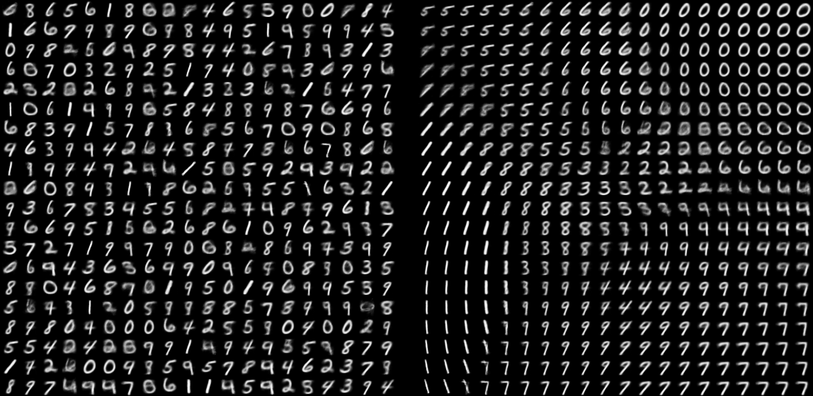
python3 vae.py --dataset=mnist --z_dim=100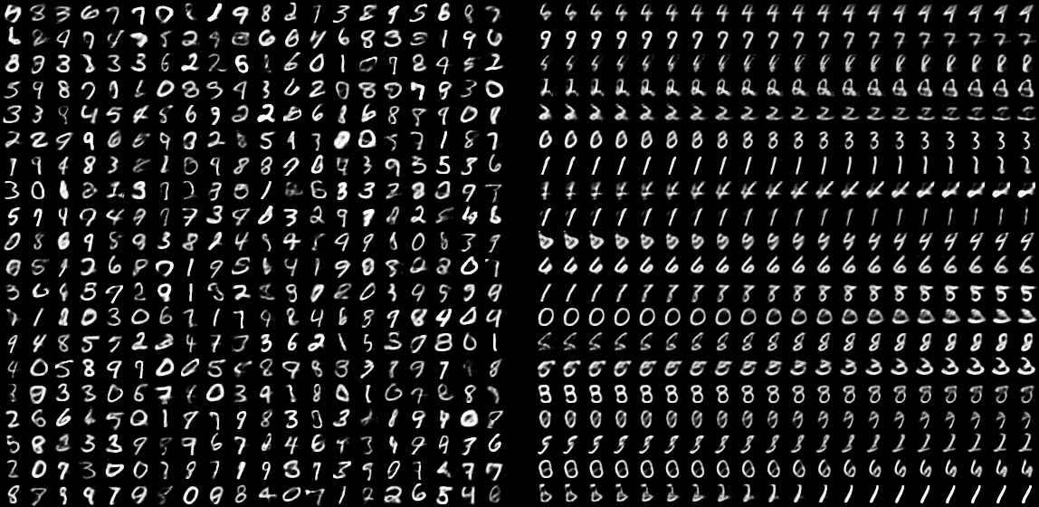
python3 vae.py --dataset=mnist-fashion --z_dim=2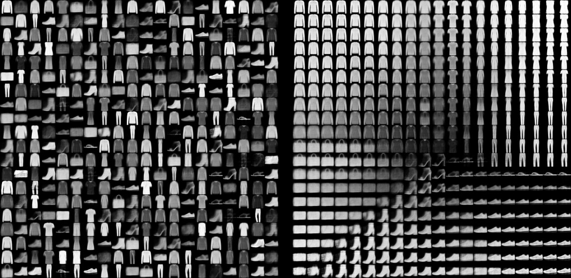
python3 vae.py --dataset=mnist-fashion --z_dim=100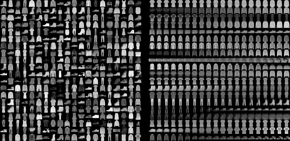
python3 vae.py --dataset=mnist-cifarcars --z_dim=2
python3 vae.py --dataset=mnist-cifarcars --z_dim=100
gan
Deadline: Jun 28, 22:00 2 points
In this assignment you will implement a simple Generative Adversarion Network for three datasets in the MNIST format. Your goal is to modify the gan.py template and implement a GAN.
After submitting the assignment to ReCodEx, you can experiment with the three
available datasets (mnist, mnist-fashion, and mnist-cifarcars) and
maybe try different latent variable dimensionality. The generated images are
available in TensorBoard logs, and the images generated by the reference
solution can be also seen in the Examples.
You can also continue with dcgan assignment.
Note that your results may be slightly different, depending on your CPU type and whether you use a GPU.
python3 gan.py --dataset=mnist --train_size=490 --epochs=5 --z_dim=2
Epoch 1/5 discriminator_accuracy: 0.8389 - discriminator_loss: 0.3185 - generator_loss: 3.8554 - loss: 3.7265
Epoch 2/5 discriminator_accuracy: 1.0000 - discriminator_loss: 0.0163 - generator_loss: 5.5732 - loss: 5.3607
Epoch 3/5 discriminator_accuracy: 0.9991 - discriminator_loss: 0.0137 - generator_loss: 6.6932 - loss: 6.4308
Epoch 4/5 discriminator_accuracy: 0.9995 - discriminator_loss: 0.0130 - generator_loss: 8.6689 - loss: 8.4075
Epoch 5/5 discriminator_accuracy: 0.9980 - discriminator_loss: 0.0203 - generator_loss: 10.1508 - loss: 9.8099
python3 gan.py --dataset=mnist --train_size=490 --epochs=5 --z_dim=100
Epoch 1/5 discriminator_accuracy: 0.8422 - discriminator_loss: 0.3254 - generator_loss: 3.3758 - loss: 3.4330
Epoch 2/5 discriminator_accuracy: 1.0000 - discriminator_loss: 0.0297 - generator_loss: 4.7812 - loss: 4.6822
Epoch 3/5 discriminator_accuracy: 1.0000 - discriminator_loss: 0.0296 - generator_loss: 5.9973 - loss: 5.7049
Epoch 4/5 discriminator_accuracy: 0.9954 - discriminator_loss: 0.0590 - generator_loss: 5.9659 - loss: 5.9170
Epoch 5/5 discriminator_accuracy: 0.9879 - discriminator_loss: 0.0903 - generator_loss: 5.6847 - loss: 5.9416
Note that your results may be slightly different, depending on your CPU type and whether you use a GPU.
python3 gan.py --dataset=mnist --z_dim=2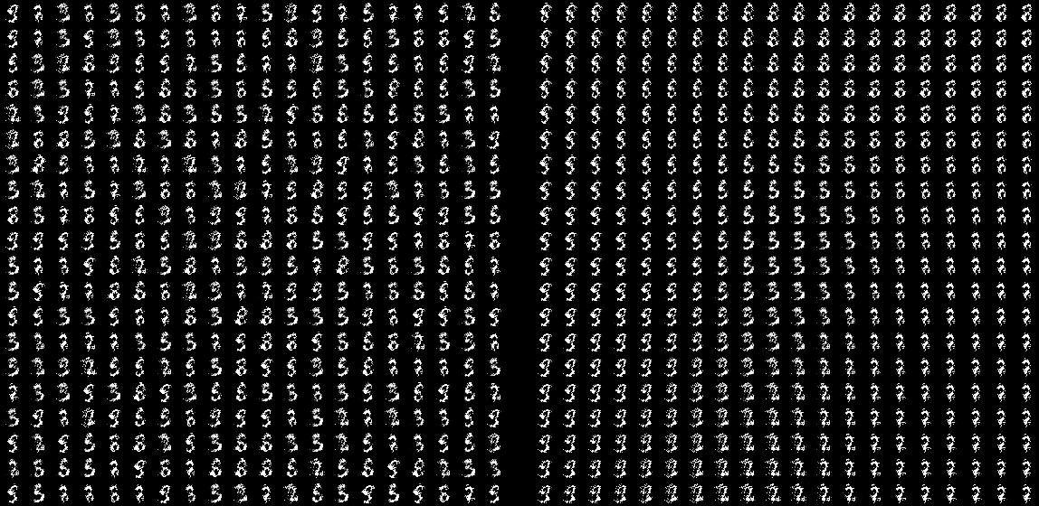
python3 gan.py --dataset=mnist --z_dim=100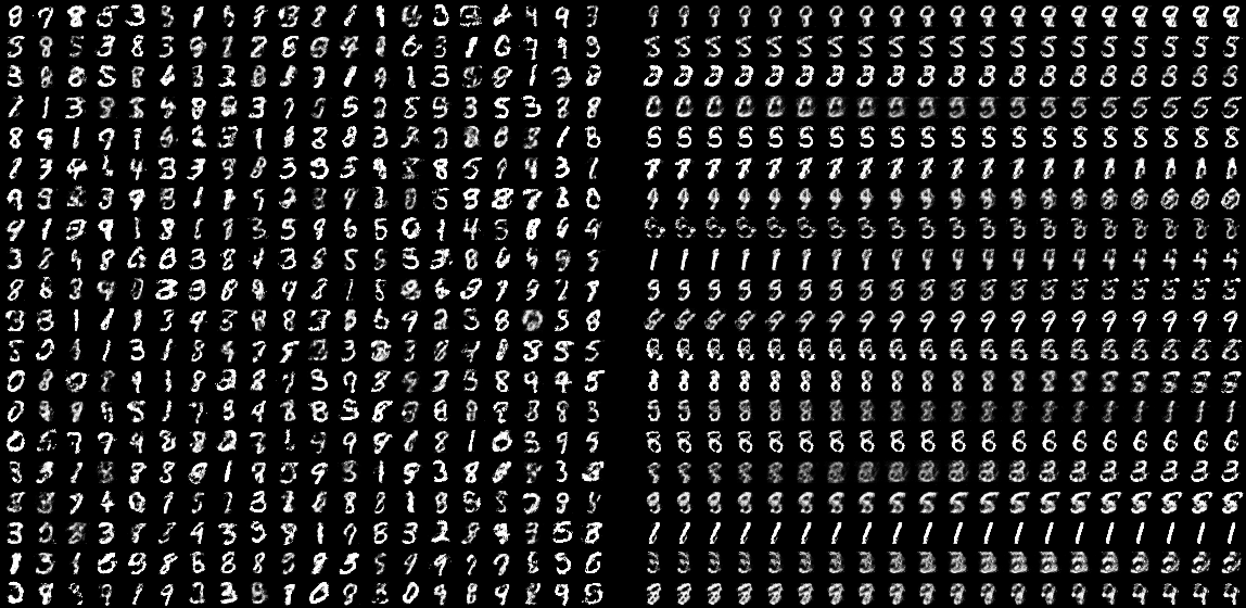
python3 gan.py --dataset=mnist-fashion --z_dim=2
python3 gan.py --dataset=mnist-fashion --z_dim=100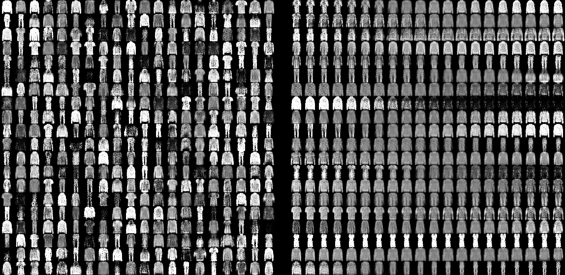
python3 gan.py --dataset=mnist-cifarcars --z_dim=2
python3 gan.py --dataset=mnist-cifarcars --z_dim=100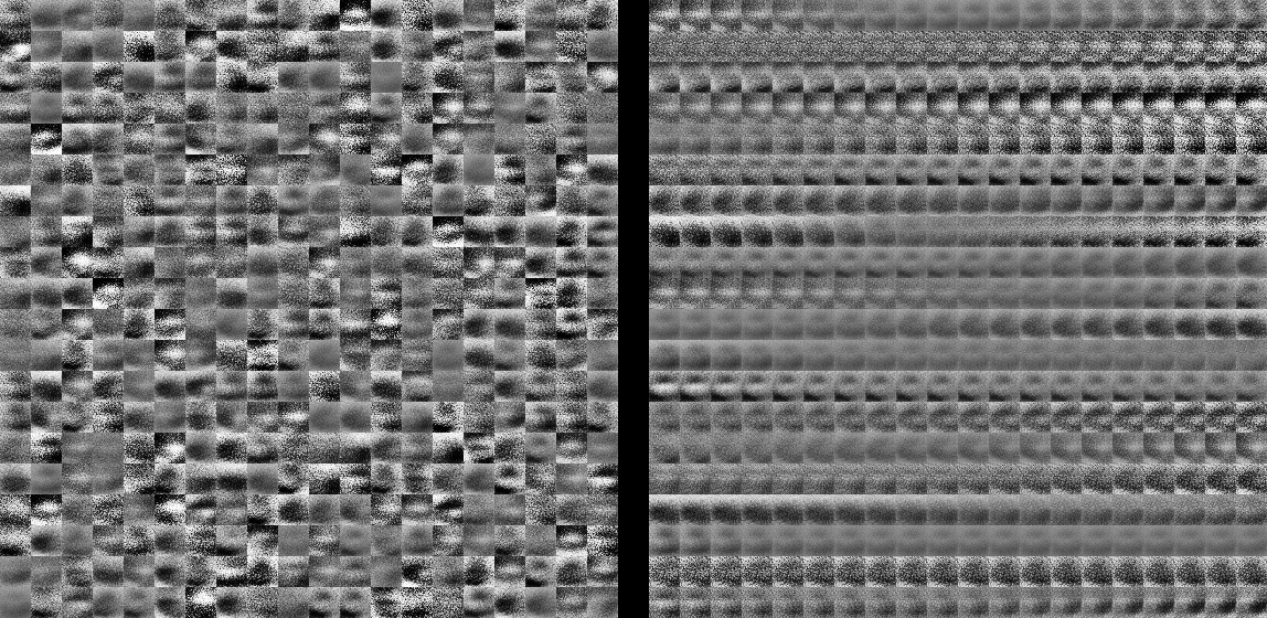
dcgan
Deadline: Jun 28, 22:00 1 points
This task is a continuation of the gan assignment, which you will modify to
implement the Deep Convolutional GAN (DCGAN).
Start with the
dcgan.py
template and implement a DCGAN. Note that most of the TODO notes are from
the gan assignment.
After submitting the assignment to ReCodEx, you can experiment with the three
available datasets (mnist, mnist-fashion, and mnist-cifarcars). However,
note that you will need a lot of computational power (preferably a GPU) to
generate the images. The generated images are available in TensorBoard logs, and
the images generated by the reference solution can be also seen in the Examples.
Note that your results may be slightly different, depending on your CPU type and whether you use a GPU.
python3 dcgan.py --dataset=mnist --train_size=490 --epochs=2 --z_dim=2
Epoch 1/2 discriminator_accuracy: 0.5139 - discriminator_loss: 2.0931 - generator_loss: 1.1888 - loss: 3.8608
Epoch 2/2 discriminator_accuracy: 0.6825 - discriminator_loss: 1.2363 - generator_loss: 0.9119 - loss: 2.1996
python3 dcgan.py --dataset=mnist --train_size=490 --epochs=2 --z_dim=100
Epoch 1/2 discriminator_accuracy: 0.5181 - discriminator_loss: 1.7983 - generator_loss: 0.9145 - loss: 2.7187
Epoch 2/2 discriminator_accuracy: 0.5873 - discriminator_loss: 1.4207 - generator_loss: 0.9856 - loss: 2.4509
Note that your results may be slightly different, depending on your CPU type and whether you use a GPU.
python3 dcgan.py --dataset=mnist --z_dim=2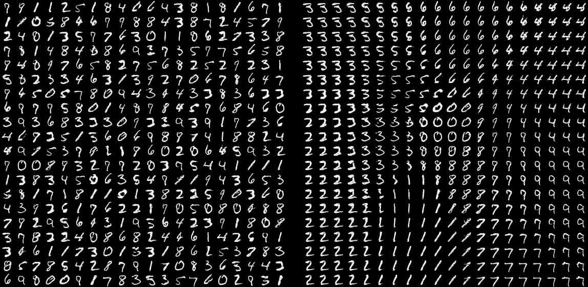
python3 dcgan.py --dataset=mnist --z_dim=100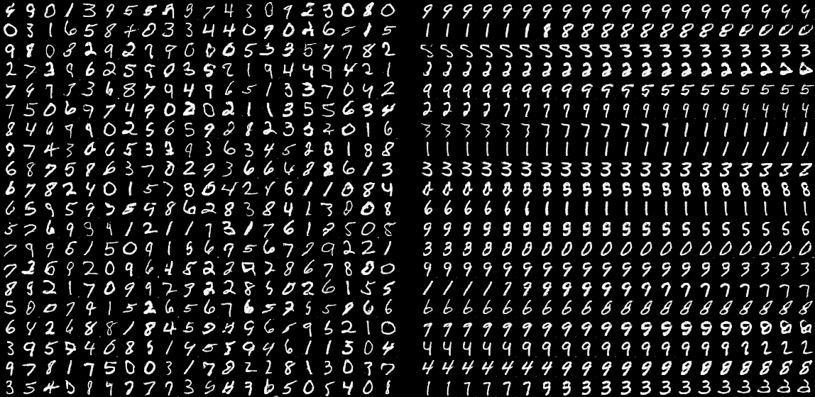
python3 dcgan.py --dataset=mnist-fashion --z_dim=2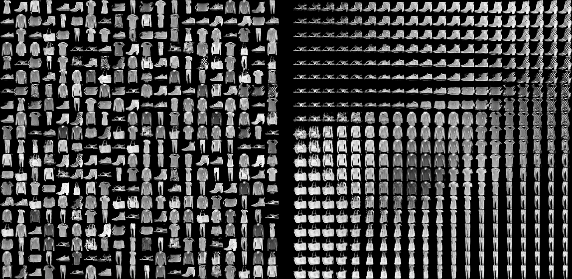
python3 dcgan.py --dataset=mnist-fashion --z_dim=100
python3 dcgan.py --dataset=mnist-cifarcars --z_dim=2
python3 dcgan.py --dataset=mnist-cifarcars --z_dim=100
ddim
Deadline: Jun 28, 22:00 3 points
Implement a Denoising Diffusion Implicit Model (DDIM) to unconditionally generate images with resolution.
The unlabeled image data can be loaded using the image64_dataset.py module, with the following datasets being available:
oxford_flowers102: 8k images of flowers, 67MB,lsun_bedrooms: 15k images of bedrooms, 109MB,ffhq: 70k images of Flickr faces, 529MB.
Start with the ddim.py
template, which contains extensive comments indicating how the architecture
should like and how the training and sampling should be performed. Note that the
template generate images to TensorBoard (after the whole training and optionally
also each --plot_each epoch), and the images generated by the reference
solution can be also seen in the Examples.
Note that your results may be slightly different, depending on your CPU type and whether you use a GPU.
python3 ddim.py --epochs=1 --epoch_batches=16 --batch_size=8 --stages=2 --stage_blocks=2 --channels=8 --ema=0.9 --sampling_steps=8
loss: 0.7859 - sample_mean: 128.2541 - sample_std: 125.8459
python3 ddim.py --epochs=1 --epoch_batches=10 --batch_size=12 --stages=3 --stage_blocks=1 --channels=12 --ema=0.8 --sampling_steps=7
loss: 0.7855 - sample_mean: 125.5367 - sample_std: 125.8327
Note that your results may be slightly different, depending on your CPU type and whether you use a GPU.
python3 ddim.py --dataset=oxford_flowers102 --epochs=70 --plot_each=10
python3 ddim.py --dataset=lsun_bedrooms --epochs=100 --plot_each=10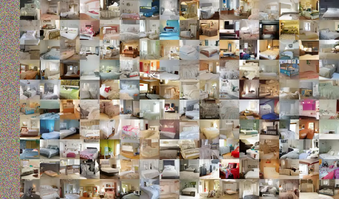
python3 ddim.py --dataset=ffhq --epochs=100 --plot_each=10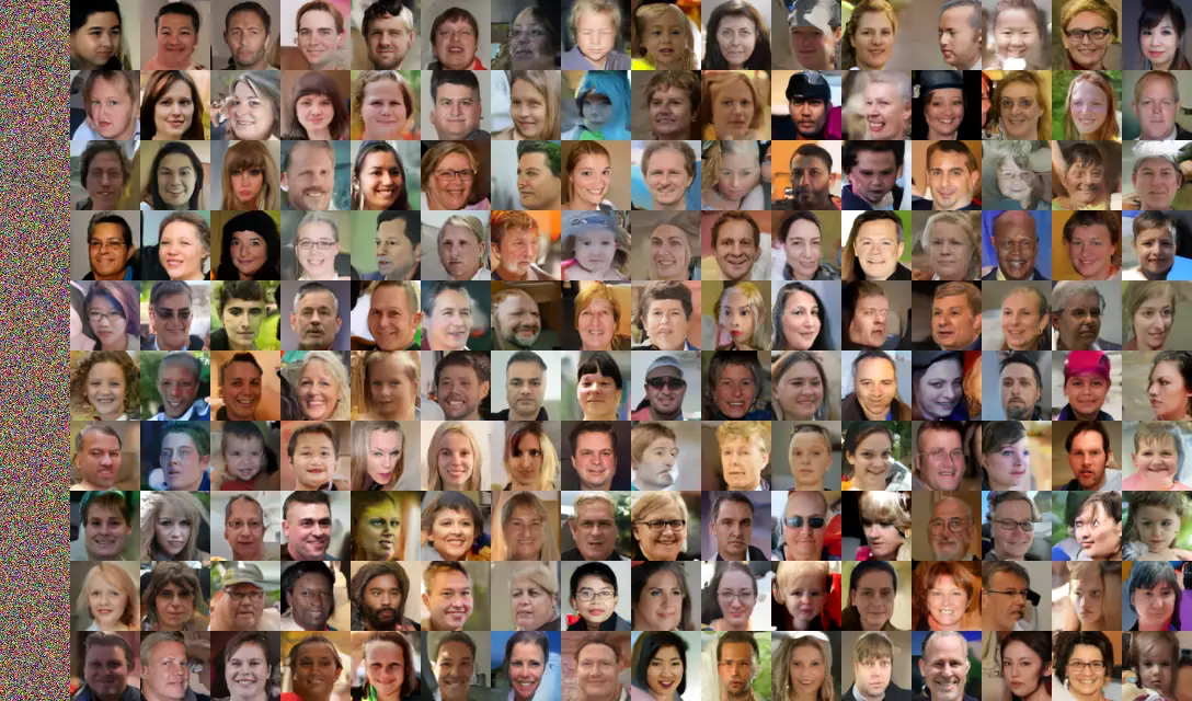
ddim_attention
Deadline: Jun 28, 22:00 1 points
This task is an extension of the ddim assignment. Your goal is
to extend the original architecture with self-attention blocks,
which are used only in some number of lower-resolution stages.
Start with the ddim_attention.py
template, where most of the comments come already from the ddim assignments.
Again, the template generate images to TensorBoard, and the images generated by
the reference solution can be also seen in the Examples.
Note that your results may be slightly different, depending on your CPU type and whether you use a GPU.
python3 ddim_attention.py --epochs=1 --epoch_batches=16 --batch_size=8 --stages=2 --stage_blocks=1 --channels=6 --ema=0.9 --sampling_steps=8 --attention_stages=0 --attention_heads=4
loss: 0.7898 - sample_mean: 124.6776 - sample_std: 125.8427
python3 ddim_attention.py --epochs=1 --epoch_batches=10 --batch_size=12 --stages=3 --stage_blocks=1 --channels=4 --ema=0.8 --sampling_steps=7 --attention_stages=1 --attention_heads=2
loss: 0.7945 - sample_mean: 126.9500 - sample_std: 125.9010
Note that your results may be slightly different, depending on your CPU type and whether you use a GPU.
python3 ddim_attention.py --dataset=oxford_flowers102 --epochs=70 --plot_each=10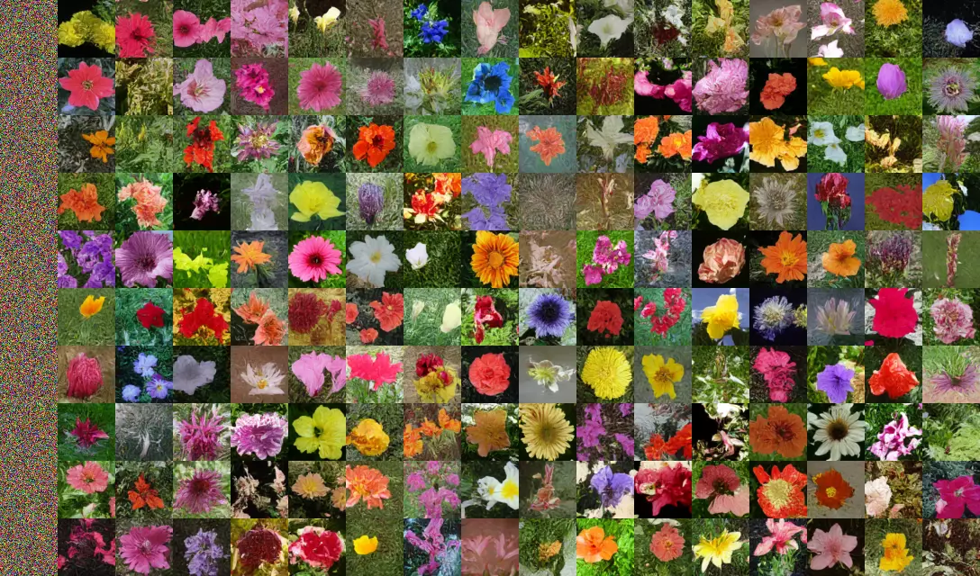
python3 ddim_attention.py --dataset=lsun_bedrooms --epochs=100 --plot_each=10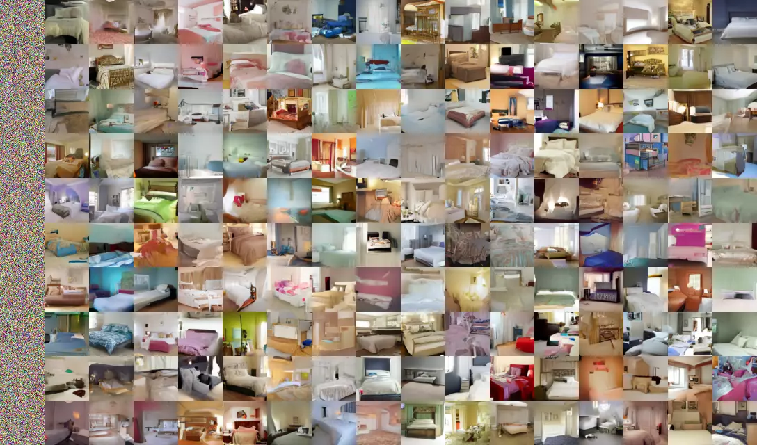
python3 ddim_attention.py --dataset=ffhq --epochs=100 --plot_each=10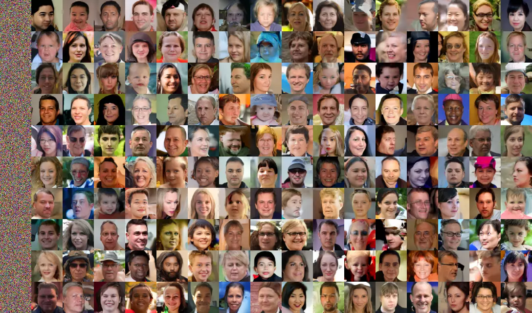
ddim_conditional
Deadline: Jun 28, 22:00 1 points
This task is an extension of the ddim assignment. Your goal is to extend the
original unconditional architecture to a conditional model, which also gets
a low-resolution version of the image to generate.
Start with the ddim_conditional.py
template, where most of the comments come already from the ddim assignments.
Again, the template generate images to TensorBoard, and the images generated by
the reference solution can be also seen in the Examples.
Note that your results may be slightly different, depending on your CPU type and whether you use a GPU.
python3 ddim_conditional.py --epochs=1 --epoch_batches=16 --batch_size=8 --stages=2 --stage_blocks=2 --channels=8 --ema=0.9 --sampling_steps=8
loss: 0.7848 - sample_mean: 112.6889 - sample_std: 100.3788
python3 ddim_conditional.py --epochs=1 --epoch_batches=10 --batch_size=12 --stages=3 --stage_blocks=1 --channels=12 --ema=0.8 --sampling_steps=7
loss: 0.7873 - sample_mean: 112.4249 - sample_std: 100.3619
Note that your results may be slightly different, depending on your CPU type and whether you use a GPU.
python3 ddim_conditional.py --dataset=oxford_flowers102 --epochs=50 --plot_each=10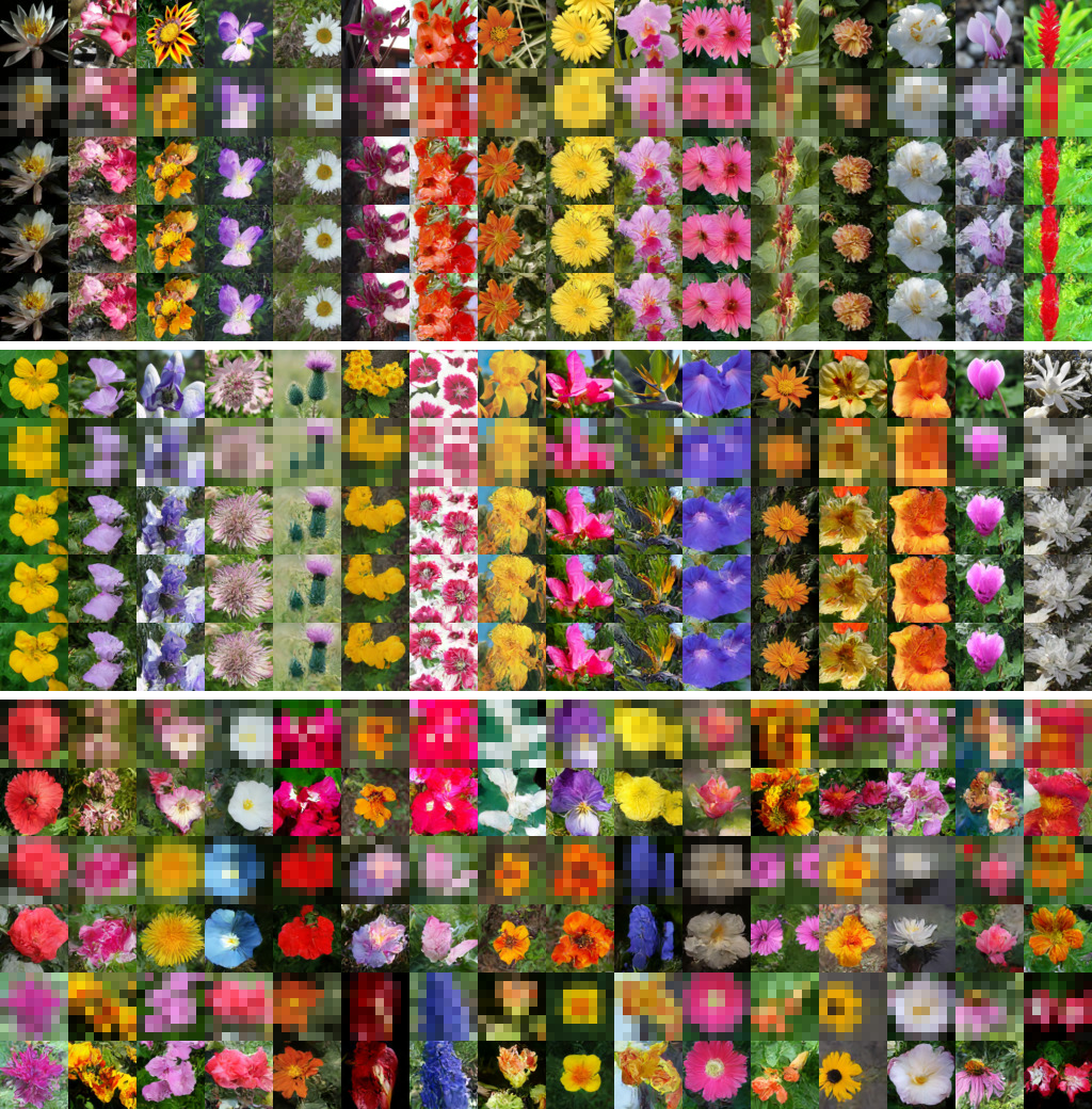
python3 ddim_conditional.py --dataset=lsun_bedrooms --epochs=50 --plot_each=10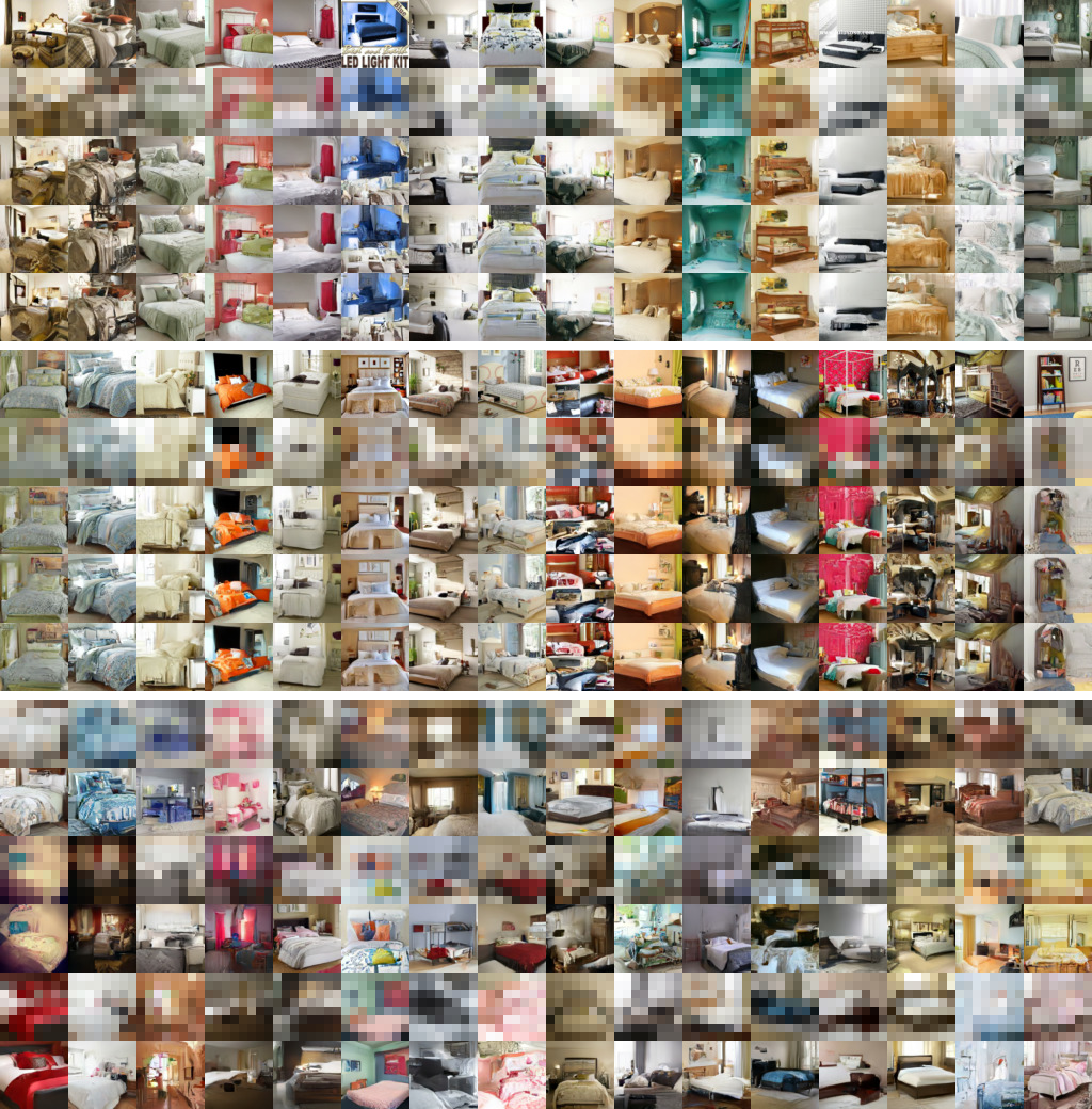
python3 ddim_conditional.py --dataset=ffhq --epochs=100 --plot_each=10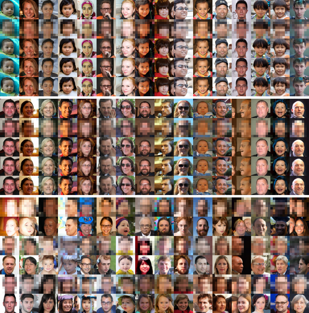
learning_to_learn
Deadline: Jun 28, 22:00 4 points
Implement a simple variant of learning-to-learn architecture using the learning_to_learn.py template. Utilizing the Omniglot dataset loadable using the omniglot_dataset.py module, the goal is to learn to classify a sequence of images using a custom hierarchy by employing external memory.
The input image sequences consist of args.classes randomly chosen Omniglot
classes, each class being assigned a randomly chosen label. For every chosen
class, args.images_per_class images are randomly selected. Apart from the
images, the input contain the random labels one step after the corresponding
images (with the first label being -1). The gold outputs are also the labels,
but without the one-step offset.
The input images should be passed through a CNN feature extraction module
and then processed using memory augmented LSTM controller; the external memory
contains enough memory cells, each with args.cell_size units. In each step,
the controller emits:
args.read_headsread keys, each used to perform a read from memory as a weighted combination of cells according to the softmax of cosine similarities of the read key and the memory cells;- a write value, which is prepended to the memory (dropping the last cell).
Note that your results may be slightly different, depending on your CPU type and whether you use a GPU.
python3 learning_to_learn.py --train_episodes=160 --test_episodes=160 --epochs=3 --classes=2
Epoch 1/3 acc: 0.5001 - acc01: 0.4920 - acc02: 0.5172 - acc05: 0.4828 - acc10: 0.4844 - loss: 0.8351 - val_acc: 0.5406 - val_acc01: 0.7469 - val_acc02: 0.6406 - val_acc05: 0.4563 - val_acc10: 0.4719 - val_loss: 0.6917
Epoch 2/3 acc: 0.5116 - acc01: 0.5288 - acc02: 0.5545 - acc05: 0.5041 - acc10: 0.4829 - loss: 0.6987 - val_acc: 0.5516 - val_acc01: 0.7250 - val_acc02: 0.6281 - val_acc05: 0.5281 - val_acc10: 0.4812 - val_loss: 0.6911
Epoch 3/3 acc: 0.5074 - acc01: 0.5530 - acc02: 0.4786 - acc05: 0.5309 - acc10: 0.5526 - loss: 0.6969 - val_acc: 0.5544 - val_acc01: 0.7500 - val_acc02: 0.6187 - val_acc05: 0.5250 - val_acc10: 0.5312 - val_loss: 0.6903
python3 learning_to_learn.py --train_episodes=160 --test_episodes=160 --epochs=3 --read_heads=2 --classes=5
Epoch 1/3 acc: 0.2060 - acc01: 0.2127 - acc02: 0.2062 - acc05: 0.2097 - acc10: 0.1997 - loss: 1.6998 - val_acc: 0.2165 - val_acc01: 0.2750 - val_acc02: 0.2338 - val_acc05: 0.2100 - val_acc10: 0.2062 - val_loss: 1.6089
Epoch 2/3 acc: 0.2088 - acc01: 0.1978 - acc02: 0.2190 - acc05: 0.2155 - acc10: 0.2173 - loss: 1.6191 - val_acc: 0.2176 - val_acc01: 0.2663 - val_acc02: 0.2362 - val_acc05: 0.2125 - val_acc10: 0.2100 - val_loss: 1.6082
Epoch 3/3 acc: 0.2067 - acc01: 0.2096 - acc02: 0.2122 - acc05: 0.2125 - acc10: 0.2114 - loss: 1.6121 - val_acc: 0.2171 - val_acc01: 0.3375 - val_acc02: 0.2425 - val_acc05: 0.2025 - val_acc10: 0.1850 - val_loss: 1.6073
Note that your results may be slightly different, depending on your CPU type and whether you use a GPU.
python3 learning_to_learn.py --epochs=50 --classes=2
Epoch 1/50 acc: 0.5611 - acc01: 0.6706 - acc02: 0.5922 - acc05: 0.5470 - acc10: 0.5286 - loss: 0.6838 - val_acc: 0.7102 - val_acc01: 0.5875 - val_acc02: 0.6625 - val_acc05: 0.7120 - val_acc10: 0.7850 - val_loss: 0.5361
Epoch 2/50 acc: 0.8047 - acc01: 0.6067 - acc02: 0.7412 - acc05: 0.8309 - acc10: 0.8573 - loss: 0.3806 - val_acc: 0.8364 - val_acc01: 0.6295 - val_acc02: 0.8075 - val_acc05: 0.8750 - val_acc10: 0.8790 - val_loss: 0.3403
Epoch 3/50 acc: 0.8885 - acc01: 0.6261 - acc02: 0.8607 - acc05: 0.9249 - acc10: 0.9296 - loss: 0.2362 - val_acc: 0.8612 - val_acc01: 0.5575 - val_acc02: 0.8320 - val_acc05: 0.9015 - val_acc10: 0.9170 - val_loss: 0.3095
Epoch 4/50 acc: 0.9165 - acc01: 0.6401 - acc02: 0.8890 - acc05: 0.9506 - acc10: 0.9627 - loss: 0.1759 - val_acc: 0.9072 - val_acc01: 0.6485 - val_acc02: 0.8875 - val_acc05: 0.9415 - val_acc10: 0.9605 - val_loss: 0.2042
Epoch 5/50 acc: 0.9327 - acc01: 0.6691 - acc02: 0.9197 - acc05: 0.9667 - acc10: 0.9732 - loss: 0.1437 - val_acc: 0.8991 - val_acc01: 0.5850 - val_acc02: 0.9005 - val_acc05: 0.9355 - val_acc10: 0.9525 - val_loss: 0.2272
Epoch 10/50 acc: 0.9489 - acc01: 0.6942 - acc02: 0.9508 - acc05: 0.9790 - acc10: 0.9824 - loss: 0.1038 - val_acc: 0.9100 - val_acc01: 0.6355 - val_acc02: 0.8875 - val_acc05: 0.9500 - val_acc10: 0.9680 - val_loss: 0.1962
Epoch 20/50 acc: 0.9585 - acc01: 0.7080 - acc02: 0.9676 - acc05: 0.9882 - acc10: 0.9917 - loss: 0.0788 - val_acc: 0.9362 - val_acc01: 0.6935 - val_acc02: 0.9300 - val_acc05: 0.9675 - val_acc10: 0.9785 - val_loss: 0.1425
Epoch 50/50 acc: 0.9663 - acc01: 0.7207 - acc02: 0.9819 - acc05: 0.9954 - acc10: 0.9961 - loss: 0.0573 - val_acc: 0.9486 - val_acc01: 0.6915 - val_acc02: 0.9550 - val_acc05: 0.9790 - val_acc10: 0.9865 - val_loss: 0.1137
python3 learning_to_learn.py --epochs=50 --read_heads=2 --classes=5
Epoch 1/50 acc: 0.2279 - acc01: 0.3091 - acc02: 0.2439 - acc05: 0.2195 - acc10: 0.2099 - loss: 1.6053 - val_acc: 0.3467 - val_acc01: 0.4224 - val_acc02: 0.3386 - val_acc05: 0.3262 - val_acc10: 0.3548 - val_loss: 1.4456
Epoch 2/50 acc: 0.5093 - acc01: 0.3486 - acc02: 0.4208 - acc05: 0.5255 - acc10: 0.5849 - loss: 1.1036 - val_acc: 0.6941 - val_acc01: 0.2430 - val_acc02: 0.5560 - val_acc05: 0.7634 - val_acc10: 0.8052 - val_loss: 0.7470
Epoch 3/50 acc: 0.7590 - acc01: 0.2540 - acc02: 0.6111 - acc05: 0.8375 - acc10: 0.8680 - loss: 0.5842 - val_acc: 0.7268 - val_acc01: 0.2454 - val_acc02: 0.5834 - val_acc05: 0.8058 - val_acc10: 0.8350 - val_loss: 0.6883
Epoch 4/50 acc: 0.8060 - acc01: 0.2715 - acc02: 0.6700 - acc05: 0.8898 - acc10: 0.9108 - loss: 0.4713 - val_acc: 0.7557 - val_acc01: 0.2686 - val_acc02: 0.6314 - val_acc05: 0.8292 - val_acc10: 0.8602 - val_loss: 0.6230
Epoch 5/50 acc: 0.8264 - acc01: 0.2786 - acc02: 0.7133 - acc05: 0.9115 - acc10: 0.9269 - loss: 0.4206 - val_acc: 0.7596 - val_acc01: 0.2610 - val_acc02: 0.6358 - val_acc05: 0.8386 - val_acc10: 0.8612 - val_loss: 0.6250
Epoch 10/50 acc: 0.8714 - acc01: 0.3127 - acc02: 0.8093 - acc05: 0.9482 - acc10: 0.9591 - loss: 0.3091 - val_acc: 0.8045 - val_acc01: 0.2998 - val_acc02: 0.7284 - val_acc05: 0.8680 - val_acc10: 0.8962 - val_loss: 0.5422
Epoch 20/50 acc: 0.9008 - acc01: 0.3432 - acc02: 0.8962 - acc05: 0.9705 - acc10: 0.9762 - loss: 0.2338 - val_acc: 0.8096 - val_acc01: 0.3052 - val_acc02: 0.7614 - val_acc05: 0.8754 - val_acc10: 0.8976 - val_loss: 0.5662
Epoch 50/50 acc: 0.9236 - acc01: 0.3911 - acc02: 0.9526 - acc05: 0.9867 - acc10: 0.9899 - loss: 0.1733 - val_acc: 0.8387 - val_acc01: 0.3372 - val_acc02: 0.8224 - val_acc05: 0.8978 - val_acc10: 0.9232 - val_loss: 0.5138
In the competitions, your goal is to train a model, and then predict target values on the given unannotated test set.
Submitting to ReCodEx
When submitting a competition solution to ReCodEx, you can include any
number of files of any kind, and either submit them individually or
compess them in a .zip file. However, there should be exactly one
text file with the test set annotation (.txt) and at least one
Python source (.py/ipynb) containing the model training and prediction.
The Python sources are not executed, but must be included for inspection.
Competition Evaluation
-
For every submission, ReCodEx checks the above conditions (exactly one
.txt, at least one.py/ipynb) and whether the given annotations can be evaluated without error. If not, it will report the corresponding error in the logs. -
Before the first deadline, ReCodEx prints the exact achieved performance, but only if it is worse than the baseline.
If you surpass the baseline, the assignment is marked as solved in ReCodEx and you immediately get regular points for the assignment. However, ReCodEx does not print the reached performance.
-
After the first deadline, the latest submission of every user surpassing the required baseline participates in a competition. Additional bonus points are then awarded according to the ordering of the performance of the participating submissions.
-
After the competition results announcement, ReCodEx starts to show the exact performance for all the already submitted solutions and also for the solutions submitted later.
What Is Allowed
- You can use only the given annotated data for training and evaluation.
- You can use the given annotated training data in any way.
- You can use the given annotated development data for evaluation or hyperparameter tuning, but not for the training itself.
- Additionally, you can use any unannotated or manually created data for training and evaluation.
- The test set annotations must be the result of your system (so you cannot manually correct them; but your system can contain other parts than just trained models, like hand-written rules).
- Do not use test set annotations in any way, if you somehow get access to them.
- Unless stated otherwise, you can use any architecture to solve the
competition task at hand, but the implementation must be created by you
and you must understand it fully. You can of course take inspiration from
any paper or existing implementation, but please reference it in that case.
- You can of course use anything from the Keras/PyTorch packages (but not models from Keras CV, torchvision, …).
- You can use any data augmentation (even implementations not written by you).
- You can use any optimizer and any hyperparameter optimization method (even implementations not written by you).
- If you utilize an already trained model, it must be trained only on the allowed training data, unless stated otherwise.
Install
-
Installing to central user packages repository
You can install all required packages to central user packages repository using
python3 -m pip install --user --no-cache-dir keras~=3.0.5 --extra-index-url=https://download.pytorch.org/whl/cu118 torch~=2.2.0 torchaudio~=2.2.0 torchvision~=0.17.0 torchmetrics~=1.3.1 flashlight-text~=0.0.3 tensorboard~=2.16.2 transformers~=4.37.2 gymnasium~=1.0.0a1 pygame~=2.5.2.The above command installs CUDA 11.8 PyTorch build, but you can change
cu118to:cputo get CPU-only (smaller) version,cu121to get CUDA 12.1 build,rocm5.7to get AMD ROCm 5.7 build.
-
Installing to a virtual environment
Python supports virtual environments, which are directories containing independent sets of installed packages. You can create a virtual environment by running
python3 -m venv VENV_DIRfollowed byVENV_DIR/bin/pip install --no-cache-dir keras~=3.0.5 --extra-index-url=https://download.pytorch.org/whl/cu118 torch~=2.2.0 torchaudio~=2.2.0 torchvision~=0.17.0 torchmetrics~=1.3.1 flashlight-text~=0.0.3 tensorboard~=2.16.2 transformers~=4.37.2 gymnasium~=1.0.0a1 pygame~=2.5.2. (orVENV_DIR/Scripts/pipon Windows).Again, apart from the CUDA 11.8 build, you can change
cu118to:cputo get CPU-only (smaller) version,cu121to get CUDA 12.1 build,rocm5.7to get AMD ROCm 5.7 build.
-
Windows installation
-
On Windows, it can happen that
python3is not in PATH, whilepycommand is – in that case you can usepy -m venv VENV_DIR, which uses the newest Python available, or for examplepy -3.11 -m venv VENV_DIR, which uses Python version 3.11. -
If you encounter a problem creating the logs in the
args.logdirdirectory, a possible cause is that the path is longer than 260 characters, which is the default maximum length of a complete path on Windows. However, you can increase this limit on Windows 10, version 1607 or later, by following the instructions.
-
-
GPU support on Linux and Windows
PyTorch supports NVIDIA GPU or AMD GPU out of the box, you just need to select appropriate
--extra-index-urlwhen installing the packages.If you encounter problems loading CUDA or cuDNN libraries, make sure your
LD_LIBRARY_PATHdoes not contain paths to older CUDA/cuDNN libraries. -
GPU support on macOS
The support for Apple Silicon GPUs in PyTorch+Keras is currently not great. Apple is working on
mlxbackend for Keras, which might improve the situation in the future.You can instead use the TensorFlow backend – just install
tensorflow~=2.16.1andtensorflow-metalpackages from PyPI, and runexport KERAS_BACKEND=tensorflowin every terminal before running assignment scripts. -
How to install TensorFlow
If you would like to install also TensorFlow, run
pip install tensorflow-cpufor CPU-only support, andpip install tensorflow[and-cuda]for Linux/WSL2 GPU support. However, the paths to the CUDA libraries seem not to be detected correctly, so I had to runexport LD_LIBRARY_PATH=$(echo VENV_DIR/lib/python*/site-packages/nvidia/*/lib | tr " " ":")in the terminal for the GPU support to work.
MetaCentrum
-
How to apply for MetaCentrum account?
After reading the Terms and conditions, you can apply for an account here.
After your account is created, please make sure that the directories containing your solutions are always private.
-
How to activate Python 3.10 on MetaCentrum?
On Metacentrum, currently the newest available Python is 3.10, which you need to activate in every session by running the following command:
module add python/python-3.10.4-intel-19.0.4-sc7snnf -
How to install the required virtual environment on MetaCentrum?
To create a virtual environment, you first need to decide where it will reside. Either you can find a permanent storage, where you have large-enough quota, or you can use scratch storage for a submitted job.
TL;DR:
-
Run an interactive CPU job, asking for 16GB scratch space:
qsub -l select=1:ncpus=1:mem=8gb:scratch_local=16gb -I -
In the job, use the allocated scratch space as the temporary directory:
export TMPDIR=$SCRATCHDIR -
You should clear the scratch space before you exit using the
clean_scratchcommand. You can instruct the shell to call it automatically by running:trap 'clean_scratch' TERM EXIT -
Finally, create the virtual environment and install PyTorch in it:
module add python/python-3.10.4-intel-19.0.4-sc7snnf
python3 -m venv CHOSEN_VENV_DIR
CHOSEN_VENV_DIR/bin/pip install --no-cache-dir --upgrade pip setuptools
CHOSEN_VENV_DIR/bin/pip install --no-cache-dir keras~=3.0.5 --extra-index-url=https://download.pytorch.org/whl/cu118 torch~=2.2.0 torchaudio~=2.2.0 torchvision~=0.17.0 torchmetrics~=1.3.1 flashlight-text~=0.0.3 tensorboard~=2.16.2 transformers~=4.37.2 gymnasium~=1.0.0a1 pygame~=2.5.2
-
-
How to run a GPU computation on MetaCentrum?
First, read the official MetaCentrum documentation: Basic terms, Run simple job, GPU computing, GPU clusters.
TL;DR: To run an interactive GPU job with 1 CPU, 1 GPU, 8GB RAM, and 16GB scatch space, run:
qsub -q gpu -l select=1:ncpus=1:ngpus=1:mem=8gb:scratch_local=16gb -ITo run a script in a non-interactive way, replace the
-Ioption with the script to be executed.If you want to run a CPU-only computation, remove the
-q gpuandngpus=1:from the above commands.
AIC
-
How to install required packages on AIC?
The Python 3.11.7 is available
/opt/python/3.11.7/bin/python3, so you should start by creating a virtual environment using/opt/python/3.11.7/bin/python3 -m venv VENV_DIRand then install the required packages in it using
VENV_DIR/bin/pip install --no-cache-dir keras~=3.0.5 --extra-index-url=https://download.pytorch.org/whl/cu118 torch~=2.2.0 torchaudio~=2.2.0 torchvision~=0.17.0 torchmetrics~=1.3.1 flashlight-text~=0.0.3 tensorboard~=2.16.2 transformers~=4.37.2 gymnasium~=1.0.0a1 pygame~=2.5.2 -
How to run a GPU computation on AIC?
First, read the official AIC documentation: Submitting CPU Jobs, Submitting GPU Jobs.
TL;DR: To run an interactive GPU job with 1 CPU, 1 GPU, and 16GB RAM, run:
srun -p gpu -c1 -G1 --mem=16G --pty bashTo run a shell script requiring a GPU in a non-interactive way, use
sbatch -p gpu -c1 -G1 --mem=16G SCRIPT_PATHIf you want to run a CPU-only computation, remove the
-p gpuand-G1from the above commands.
Git
-
Is it possible to keep the solutions in a Git repository?
Definitely. Keeping the solutions in a branch of your repository, where you merge them with the course repository, is probably a good idea. However, please keep the cloned repository with your solutions private.
-
On GitHub, do not create a public fork with your solutions
If you keep your solutions in a GitHub repository, please do not create a clone of the repository by using the Fork button – this way, the cloned repository would be public.
Of course, if you just want to create a pull request, GitHub requires a public fork and that is fine – just do not store your solutions in it.
-
How to clone the course repository?
To clone the course repository, run
git clone https://github.com/ufal/npfl138This creates the repository in the
npfl138subdirectory; if you want a different name, add it as a last parameter.To update the repository, run
git pullinside the repository directory. -
How to keep the course repository as a branch in your repository?
If you want to store the course repository just in a local branch of your existing repository, you can run the following command while in it:
git remote add upstream https://github.com/ufal/npfl138
git fetch upstream
git checkout -t upstream/master
This creates a branch
master; if you want a different name, add-b BRANCH_NAMEto the last command.In both cases, you can update your checkout by running
git pullwhile in it. -
How to merge the course repository with your modifications?
If you want to store your solutions in a branch merged with the course repository, you should start by
git remote add upstream https://github.com/ufal/npfl138
git pull upstream master
which creates a branch
master; if you want a different name, change the last argument tomaster:BRANCH_NAME.You can then commit to this branch and push it to your repository.
To merge the current course repository with your branch, run
git merge upstream masterwhile in your branch. Of course, it might be necessary to resolve conflicts if both you and I modified the same place in the templates.
ReCodEx
-
What files can be submitted to ReCodEx?
You can submit multiple files of any type to ReCodEx. There is a limit of 20 files per submission, with a total size of 20MB.
-
What file does ReCodEx execute and what arguments does it use?
Exactly one file with
pysuffix must contain a line starting withdef main(. Such a file is imported by ReCodEx and themainmethod is executed (during the import,__name__ == "__recodex__").The file must also export an argument parser called
parser. ReCodEx uses its arguments and default values, but it overwrites some of the arguments depending on the test being executed – the template should always indicate which arguments are set by ReCodEx and which are left intact. -
What are the time and memory limits?
The memory limit during evaluation is 1.5GB. The time limit varies, but it should be at least 10 seconds and at least twice the running time of my solution.
Finetuning
-
How to make a part of the network frozen, so that its weights are not updated?
Each
keras.layers.Layer/keras.Modelhas a mutabletrainableproperty indicating whether its variables should be updated – however, after changing it, you need to call.compileagain (or otherwise make sure the list of trainable variables for the optimizer is updated).Note that once
trainable == False, the insides of a layer are no longer considered, even if some its sub-layers havetrainable == True. Therefore, if you want to freeze only some sub-layers of a layer you use in your model, the layer itself must havetrainable == True. -
How to choose whether dropout/batch normalization is executed in training or inference regime?
When calling a
keras.layers.Layer/keras.Model, a named optiontrainingcan be specified, indicating whether training or inference regime should be used. For a model, this option is automatically passed to its layers which require it, and Keras automatically passes it duringmodel.{fit,evaluate,predict}.However, you can manually pass for example
training=Falseto a layer when using Functional API, meaning that layer is executed in the inference regime even when the whole model is training. -
How does
trainableandtraininginteract?The only layer, which is influenced by both these options, is batch normalization, for which:
- if
trainable == False, the layer is always executed in inference regime; - if
trainable == True, the training/inference regime is chosen according to thetrainingoption.
- if
TensorBoard
-
Cannot start TensorBoard after installation
If
tensorboardexecutable cannot be found, make sure the directory with pip installed packages is in your PATH (that directory is either in your virtual environment if you use a virtual environment, or it should be~/.local/binon Linux and%UserProfile%\AppData\Roaming\Python\Python311and%UserProfile%\AppData\Roaming\Python\Python311\Scriptson Windows). -
What can be logged in TensorBoard? See the documentation of the
SummaryWriter. Common possibilities are:- scalar values:
summary_writer.add_scalar(name like "train/loss", value, step) - tensor values displayed as histograms or distributions:
summary_writer.add_histogram(name like "train/output_layer", tensor, step) - images as tensors with shape
[num_images, h, w, channels], wherechannelscan be 1 (grayscale), 2 (grayscale + alpha), 3 (RGB), 4 (RGBA):summary_writer.add_images(name like "train/samples", images, step, dataformats="NHWC")"HWC"(shape[h, w, channels]),"HW","NCHW","CHW". - possibly large amount of text (e.g., all hyperparameter values, sample
translations in MT, …) in Markdown format:
summary_writer.add_text(name like "hyperparameters", markdown, step) - audio as tensors with shape
[1, samples]and values in range:summary_writer.add_audio(name like "train/samples", clip, step, [sample_rate])
- scalar values:
Requirements
To pass the practicals, you need to obtain at least 80 points, excluding the bonus points. Note that all surplus points (both bonus and non-bonus) will be transfered to the exam. In total, assignments for at least 120 points (not including the bonus points) will be available, and if you solve all the assignments (any non-zero amount of points counts as solved), you automatically pass the exam with grade 1.
To pass the exam, you need to obtain at least 60, 75, or 90 points out of 100-point exam to receive a grade 3, 2, or 1, respectively. The exam consists of 100-point-worth questions from the list below (the questions are randomly generated, but in such a way that there is at least one question from every but the first lecture). In addition, you can get surplus points from the practicals and at most 10 points for community work (i.e., fixing slides or reporting issues) – but only the points you already have at the time of the exam count. You can take the exam without passing the practicals first.
Exam Questions
Lecture 1 Questions
-
Considering a neural network with input neurons, a single hidden layer with neurons, output neurons, hidden activation and output activation , list its parameters (including their size) and write down how the output is computed. [5]
-
List the definitions of frequently used MLP output layer activations (the ones producing parameters of a Bernoulli distribution and a categorical distribution). Then write down three commonly used hidden layer activations (sigmoid, tanh, ReLU). [5]
-
Formulate the Universal approximation theorem. [5]
Lecture 2 Questions
-
Define maximum likelihood estimation, and show that it is equal to minimizing NLL, minimizing cross-entropy, and minimizing KL divergence. [10]
-
Define mean squared error, show how it can be derived using MLE (define , show how MLE looks using , and prove that the maximum likelihood estimate is equal to minimizing MSE). [5]
-
Describe gradient descent and compare it to stochastic (i.e., online) gradient descent and minibatch stochastic gradient descent. [5]
-
Formulate conditions on the sequence of learning rates used in SGD to converge to optimum almost surely. [5]
-
Write down the backpropagation algorithm. [5]
-
Write down the mini-batch SGD algorithm with momentum. [5]
-
Write down the AdaGrad algorithm and show that it tends to internally decay learning rate by a factor of in step . Then write down the RMSProp algorithm and explain how it solves the problem with the involuntary learning rate decay. [10]
-
Write down the Adam algorithm. Then show why the bias-correction terms make the estimation of the first and second moment unbiased. [10]
Lecture 3 Questions
-
Considering a neural network with input neurons, a single ReLU hidden layer with units and softmax output layer with units, write down the explicit formulas (i.e., without differential operators) of the gradient of all the MLP parameters (two weight matrices and two bias vectors), assuming input , target and negative log likelihood loss. [10]
-
Assume a network with MSE loss generated a single output , and the target output is . What is the value of the loss function itself, and what is the explicit formula (i.e., without a differential operator) of the gradient of the loss function with respect to ? [5]
-
Assume a binary-classification network with cross-entropy loss generated a single output , which is passed through the sigmoid output activation function, producing . If the target output is , what is the value of the loss function itself, and what is the explicit formula (i.e., without a differential operator) of the gradient of the loss function with respect to ? [5]
-
Assume a -class-classification network with cross-entropy loss generated a -element output , which is passed through the softmax output activation function, producing . If the target distribution is , what is the value of the loss function itself, and what is the explicit formula (i.e., without a differential operator) of the gradient of the loss function with respect to ? [5]
-
Define regularization and describe its effect both on the value of the loss function and on the value of the loss function gradient. [5]
-
Describe the dropout method and write down exactly how it is used during training and during inference. [5]
-
Describe how label smoothing works for cross-entropy loss, both for sigmoid and softmax activations. [5]
-
How are weights and biases initialized using the default Glorot initialization? [5]
Lecture 4 Questions
-
Write down the equation of how convolution of a given image is computed. Assume the input is an image of size with channels, the kernel has size , the stride is , the operation performed is in fact cross-correlation (as usual in convolutional neural networks) and that output channels are computed. [5]
-
Explain both
SAMEandVALIDpadding schemes and write down the output size of a convolutional operation with an kernel on image of size for both these padding schemes (stride is 1). [5] -
Describe batch normalization including all its parameters, and write down an algorithm how it is used during training and the algorithm how it is used during inference. Be sure to explicitly write over what is being normalized in case of fully connected layers and in case of convolutional layers. [10]
-
Describe overall architecture of VGG-19 (you do not need to remember the exact number of layers/filters, but you should describe the overall order and type of layers that are used). [5]
Lecture 5 Questions
-
Describe overall architecture of ResNet. You do not need to remember the exact number of layers/filters, but you should draw a bottleneck block (including the applications of BatchNorms and ReLUs) and state how residual connections work when the number of channels increases. [10]
-
Draw the original ResNet block (including the exact positions of BatchNorms and ReLUs) and also the improved variant with full pre-activation. [5]
-
Compare the bottleneck block of ResNet and ResNeXt architectures (draw the latter using convolutions only, i.e., do not use grouped convolutions). [5]
-
Describe the CNN regularization method of networks with stochastic depth. [5]
-
Compare Cutout and DropBlock. [5]
-
Describe in detail how is CutMix performed. [5]
-
Describe Squeeze and Excitation applied to a ResNet block. [5]
-
Draw the Mobile inverted bottleneck block (including explanation of separable convolutions, the expansion factor, exact positions of BatchNorms and ReLUs, but without describing Squeeze and excitation blocks). [5]
-
Assume an input image of size with channels, and a convolutional kernel with size , stride and output channels. Write down (or derive) the equation of transposed convolution (or equivalently backpropagation through a convolution to its inputs). [5]
Lecture 6 Questions
-
Describe the differences among semantic segmentation, image classification, object detection, and instance segmentation, and write down which metrics are used for these tasks. [5]
-
Write down how is computed given predicted objects and their bounding boxes in the whole dataset. [5]
-
Considering a Fast-RCNN architecture, draw overall network architecture, explain what a RoI-pooling layer is, show how the network parametrizes bounding boxes and write down the complete loss. Finally, describe non-maximum suppression and how the Fast-RCNN prediction is performed. [10]
-
Considering a Faster-RCNN architecture, describe the region proposal network (what are anchors, architecture including both heads, how are the coordinates of proposals parametrized, what does the complete loss look like). [10]
-
Considering Mask-RCNN architecture, describe the additions to a Faster-RCNN architecture (the RoI-Align layer, the new mask-producing head, its loss). [5]
-
Write down the focal loss with class weighting, including the commonly used hyperparameter values and how the class weighting works for a given class. [5]
-
Draw the overall architecture of a RetinaNet architecture (the computation of , the FPN architecture computing including the block combining feature maps of different resolutions; the classification and bounding box generation heads, including their output size). Write down the losses for both heads and the overall loss. [10]
-
Describe GroupNorm (including its parameters and their size), and compare it to BatchNorm and LayerNorm, discussing both fully connected layers and convolutional layers. [5]
Lecture 8 Questions
-
Write down how the Long Short-Term Memory (LSTM) cell operates, including the explicit formulas. Also mention the forget gate bias. [10]
-
Write down how the Gated Recurrent Unit (GRU) operates, including the explicit formulas. [10]
-
Describe Highway network computation. [5]
-
Why the usual dropout cannot be used on recurrent state? Describe how the problem can be alleviated with variational dropout. [5]
-
Describe layer normalization including all its parameters, and write down how it is computed (be sure to explicitly state over what is being normalized in case of fully connected layers and convolutional layers). [5]
-
Draw a tagger architecture utilizing word embeddings, recurrent character-level word embeddings (including how are these computed from individual characters), and two sentence-level bidirectional RNNs (explaining the bidirectionality) with a residual connection. Where would you put the dropout layers? [10]
Lecture 9 Questions
-
In the context of named entity recognition, describe what the BIO encoding is and why it is used. [5]
-
Write down the dynamic programming algorithm for decoding a BIO-tag sequence, including its asymptotic complexity. [10]
-
In the context of CTC loss, describe regular and extended labelings and write down the algorithm for computing the log probability of a gold label sequence . [10]
-
Describe how CTC predictions are performed using a beam-search. [5]
-
Draw the CBOW architecture from
word2vec, including the sizes of the inputs and the sizes of the outputs and used non-linearities. Also make sure to indicate where the embeddings are being trained. [5] -
Draw the SkipGram architecture from
word2vec, including the sizes of the inputs and the sizes of the outputs and used non-linearities. Also make sure to indicate where the embeddings are being trained. [5] -
Describe the hierarchical softmax used in
word2vec. [5] -
Describe the negative sampling proposed in
word2vec, including the choice of distribution of negative samples. [5] -
Explain how are ELMo embeddings trained and how are they used in downstream applications. [5]
Lecture 10 Questions
-
Considering machine translation, draw a recurrent sequence-to-sequence architecture without attention, both during training and during inference (include embedding layers, recurrent cells, classification layers, argmax/softmax). [5]
-
Considering machine translation, draw a recurrent sequence-to-sequence architecture with attention, used during training (include embedding layers, recurrent cells, attention, classification layers). Then write down how exactly is the attention computed. [10]
-
Explain how is word embeddings tying used in a sequence-to-sequence architecture, including the necessary scaling. [5]
-
Write down why are subword units used in text processing, and describe the BPE algorithm for constructing a subword dictionary from a large corpus. [5]
-
Write down why are subword units used in text processing, and describe the WordPieces algorithm for constructing a subword dictionary from a large corpus. [5]
-
Pinpoint the differences between the BPE and WordPieces algorithms, both during dictionary construction and during inference. [5]
-
Describe the Transformer encoder architecture, including the description of self-attention (but you do not need to describe multi-head attention), FFN and positions of LNs and dropouts. [10]
-
Write down the formula of Transformer self-attention assuming you get sequence representation , and then describe multi-head self-attention in detail, including the dimensionality of the individual heads. [10]
-
Describe the Transformer decoder architecture, including the description of self-attention and masked self-attention (but you do not need to describe multi-head attention), FFN and positions of LNs and dropouts. Also discuss the difference between training and prediction regimes. [10]
Lecture 11 Questions
-
Why are positional embeddings needed in Transformer architecture? Write down the sinusoidal positional embeddings used in the Transformer. [5]
-
Compare RNN to Transformer – what are the strengths and weaknesses of these architectures? [5]
-
Describe the BERT architecture (you do not need to describe the (multi-head) self-attention operation). Elaborate also on which positional embeddings are used and what are the GELU activations. [10]
-
Describe the GELU activations and explain why are they a combination of ReLUs and Dropout. [5]
-
Elaborate on BERT training process (what are the two objectives used and how exactly are the corresponding losses computed). [10]
-
Describe the architecture of a Vision Transformer – how are input images represented, draw the Transformer encoder layer and the FFN sublayer, how is the distribution over predicted classes computed, what positional embeddings are used (and what alternative positional embeddings were tried). [10]
Lecture 12 Questions
-
Define the Markov Decision Process, including the definition of the return. [5]
-
Define the value function, such that all expectations are over simple random variables (actions, states, rewards), not trajectories. [5]
-
Define the action-value function, such that all expectations are over simple random variables (actions, states, rewards), not trajectories. [5]
-
Express the value function using the action-value function, and express the action-value function using the value function. [5]
-
Formulate the policy gradient theorem. [5]
-
Prove the part of the policy gradient theorem showing the value of . [10]
-
Assuming the policy gradient theorem, formulate the loss used by the REINFORCE algorithm and show how can its gradient be expressed as an expectation over states and actions. [5]
-
Write down the REINFORCE algorithm, including the loss formula. [10]
-
Show that introducing baseline does not influence validity of the policy gradient theorem. [5]
-
Write down the REINFORCE with baseline algorithm, including both loss formulas. [10]
-
Sketch the overall structure and training procedure of the Neural Architecture Search. You do not need to describe how exactly is the block produced by the controller. [5]
-
Write down the variational lower bound (ELBO) in the form of a reconstruction error minus the KL divergence between the encoder and the prior (i.e., in the form used for model training). Then prove it is actually a lower bound on the log-likelihood . [10]
-
Draw an architecture of a variational autoencoder (VAE). Pay attention to the parametrization of the distribution from the encoder (including the used activation functions), show how to perform latent variable sampling so that it is differentiable with respect to the encoder parameters (the reparametrization trick), and write down the loss. [10]
Lecture 13 Questions
-
Write down the min-max formulation of generative adversarial network (GAN) objective. Then describe what loss is actually used for training the generator in order to avoid vanishing gradients at the beginning of the training. [5]
-
Write down the training algorithm of generative adversarial networks (GAN), including the losses minimized by the discriminator and the generator. Be sure to use the version of generator loss which avoids vanishing gradients at the beginning of the training. [10]
-
Explain how the class label is used when training a conditional generative adversarial network (CGAN). [5]
-
Illustrate that alternating SGD steps are not guaranteed to converge for a min-max problem. [5]
-
Assuming a data point and a variance schedule , define the forward diffusion process . [5]
-
Assuming a variance schedule , prove how the forward diffusion marginal looks like. [10]
-
Write down the diffusion marginal and the formulas of the cosine schedule of the signal rate and the noise rate. [5]
-
Write down the DDPM training algorithm, including the formula of the loss. [5]
-
Specify the inputs and outputs of the DDPM model, and describe its architecture – what the overall structure looks like (ResNet blocks, downsampling and upsampling, self-attention blocks), how the time is represented, and how the conditioning on an input image and an input text looks like. [10]
-
Define the forward DDIM process, so , , , and show how its forward diffusion marginal looks like. [5]
-
Write down the DDIM sampling algorithm. [5]
Lecture 14 Questions
-
Draw the WaveNet architecture (show the overall architecture, explain dilated convolutions, write down the gated activations, describe global and local conditioning). [10]
-
Define the Mixture of Logistic distribution used in Parallel WaveNet, including the explicit formula of computing the likelihood of the data. [5]
-
Describe the changes in the Student model of Parallel WaveNet, which allow efficient sampling (how the latent prior looks like, how the output data distribution is modeled in a single iteration, how is every iteration computed). [5]
-
Write down the loss used for training of the Student model in Parallel WaveNet, then rewrite the cross-entropy part to a sum of per-time-step cross-entropies, and explain how are the per-time-step cross-entropies estimated. [10]
-
Describe the addressing mechanism used in Neural Turing Machines – show the overall structure including the required parameters, and explain content addressing, interpolation with location addressing, shifting and sharpening. [10]
-
Explain the overall architecture of a Neural Turing Machine with an LSTM controller, assuming reading heads and one write head. Describe the inputs and outputs of the LSTM controller itself, then how the memory is read from and written to, and how the final output is computed. You do not need to write down the implementation of the addressing mechanism (you can assume it is a function which gets parameters, memory and previous distribution, and computes a new distribution over memory cells). [10]