
Table of Contents
- Introduction
- Basic concepts
- Tutorial
- Getting started
- A simple query
- A query with two nodes
- Disjunctions, regular expressions and set enumerations
- Types of relations (links)
- Querying labeled references using the
memberselector - Subqueries (testing existence, non-existence and number of occurrences)
- Looking for small result trees?
- Functions
- Output filters
- User Interfaces
- Query Language
- Installing PML-TQ server
- Tools
PML Tree Query (PML-TQ) is a query language and search engine targeted for querying multi-layer annotated treebanks stored in the PML data format. It can be used to query all kinds of treebanks: dependency, constituency, multi-layered, parallel treebanks, as well as other kinds of richly structured types of annotation.
The query language is declarative and offers both textual and graphical representation of queries. Currently, there are two implementations of the query engine, one based on a relational database (Oracle or PostgreSQL >= 8.4), the other based on Perl and the TrEd toolkit. Three user interfaces are available: a WEB-based interface for the database-based query engine displaying query results as SVG, a full-featured graphical user interface for both engines available as a plug-in to the tree editor TrEd, and a text-only command-line interface.
Main features:
queries can span over all layers of annotation (including annotation dictionaries)
allows arbitrary logical constraints
supports output filters (generate custom text output, compute statistics, ...)
offers graphical query representation with relations (links) between nodes depicted as arrows
GUI interface built into TrEd
understands PML data model (no conversion, no information loss)
TODO: comparison with other query languages and engines (NetGraph, TGrep2, TigerSearch, Nite, XPath, LPath+)
A PML-TQ query consists of a selective part that selects nodes from the treebank and an optional sequence of output filters that are used to extract data from the matching nodes, post-process the results, compute statistics, generate tabular output, etc.
The selective part of a PML-TQ query postulates requirements on one or more nodes from the treebank and their mutual relationships (e.g. on the topological configuration in the tree structure). It is formed by one or more node selectors, which form the outermost scope of the query. Inner scopes of the query are given by nested subqueries as described later.
A node selector represents a node in the treebank of a certain type (in the PML data model, the nodes in the treebank annotation can be typed; the query can also refer to several annotation layers with different types of nodes) and postulates constraints on its properties including relationships to nodes represented by other selectors.
Selectors may nest other selectors; a nested
selector belongs to the same scope as the containing selector The nested
selector may explicitly specify the relation of its matching node to the
node matched by the containing selector; the default relation is
child. The nesting of selectors can thus naturally
follow the topology of the matching tree.
Selectors can also be named and referred to from other node selectors; however, in many cases, the need for explicitly naming them can be eliminated by nesting.
A match of a query is a mapping which assigns to each outermost-scoped selector a node from a treebank (called a matching node) of the type specified by the selector, in such a way that all the matching nodes are mutually distinct and simultaneously satisfy the constraints postulated by their corresponding selectors (including constraints on their mutual relationships). The match can be represented as a tuple of the matching nodes ordered accordingly to some canonical ordering of the selectors from the outermost scope of the query. There can be zero, one, or more distinct matches of the query in the treebank (two matches are distinct if, as ordered tuples, they differ in at least one node).
Non-identity rule: Two distinct selectors in the same scope of the query always represent two distinct nodes in each match of the query or sub-query.
Selectors can postulate the following types of constraints:
predicates
references to other selectors
subqueries
boolean combinations of the above
In the following descriptions, we refer to the selector postulating a constraint as as the current selector.
Predicate constraints assert equality,
inequality, or regular expression match between values computed from
terms. An atomic term is a constant (integer, float, or character string),
or an attribute of a node matched by the current selector or some other
selector in the current or outer scope of the query. A term is either an
atomic term or a term obtained from other terms using arithmetical
(+, *, -, div, mod) or string (concatenation
& ) operators, or functions.
A reference is a constraint on the relationship of a node matched by some named selector to the node matched by the current selector. The referred selector must either belong to the same scope as the current selector or to its outer scope.
A subquery is formed by a selector (called the leading selector of the subquery) nested in the current selector and augmented by restrictions on the number of occurrences, computed as the number of distinct nodes matched by the leading selector of the subquery relatively to a fixed match of the selectors in the current and outer scope (including the current selector). For example, to postulate a constraint that each node matched by the current selector must have at least two child nodes, we create a subquery in form of a nested selector in the child relation to the current selector and restrict the number of occurrences to two and more.
The leading selector can nest other selectors. Each subquery starts a new scope whose outer scope is the scope of the containing selector together with the containing selector's outer scope (if any). Unlike selectors from the outermost scope, selectors declared within a subquery do not represent any particular node in the resulting match. They can refer to selectors from the same scope, and also to selectors from the outer scope, but not vice versa (selectors from the outer scope cannot refer to the selectors in the subquery).
A subquery constraint is verified as follows: for each match of the selectors in the current and outer scope, all matches of the subquery are located (these may coincide with nodes matched by the selectors in the outer scope). The number of distinct nodes matched by the leading selector of the subquery are counted and this number is compared with the restrictions on number of occurrences. The constraint is satisfied if and only if these restrictions are met.
A constraint can also be a boolean combination of other constraints; a nested node selector occurring in a boolean combination with other nested node selectors or constraints is considered to be a subquery with at least one occurrence.
A PML-TQ query can be visualized as a graph consisting of one or more trees whose nodes are the selectors connected by edges according to the nesting of selectors and subqueries. In this sense we may sometimes refer to selectors as query nodes and to the query as query graph or query tree (a technical root can be added above all the trees so that a forest becomes a single tree). The edges can be labeled or colored to represent different relationships between nodes. References to named selectors can be represented by an additional layer of links (edges) in the graph that may go across the basic tree structure of the query tree.
The purpose of this tutorial is to show how to create and run queries from the tree editor TrEd. The textual form of the query can also be used in the web or command-line interface.
As our examples, we use queries over the Prague Dependency Treebank 2.0; conceptually similar queries can be applied to most other treebanks, although the node types and attributes will be probably different.
The tutorial gradually passes from very simple to complex queries and demonstrates various common syntactic constructions of the PML-TQ language. We always show how to write the query in the textual form as well as how to build and run the query graphically in the tree editor TrEd.
To start using PML-TQ from the tree editor TrEd, press Shift+F3 or select → → from the main menu in TrEd.

Choose ; if
doing this for the first time, you will be asked to fill the connection
form: as url, fill the search engine URL including
port number (e.g. http://mysearchserver.org:8082
where mysearchserver.org is the host name or
IP address of your PML-TQ search service and
8082 is the port the search service is
listening on); fill username and
password with your credentials for the search service
(which you can receive from the administrator of the PML-TQ search
service). When done, confirm with OK. TrEd will
attempt to contact the search service you have specified and will ask it
for a list of treebanks avaiable. Subsequently, you will be asked to
select treebanks for which you want to configure a connection.
Once your connections are configured, a dialog window with a list
of available connections will be offered. To select a connection, simply
choose it from the list and press . You may
also use the buttons to add/remove
connections to other treebanks provided by the server of the selected
connection, to create a connection to a
new server, to display information about the
selected connection (such as name and description of the treebank),
to modify the connection data
(url, username, and
password), and to
remove the selected connection from the list.
A window with an empty query tree is displayed by TrEd:
You can also use the toolkit without TrEd from a web browser (although you will not be able to build the query graphically nor see the graphical representation of your query). To start, just open the search engine URL and log in using any web browser capable of combining JavaScript, CSS, and SVG (Scalable Vector Graphics). At the time of writing this tutorial, the best choice is the Opera browser, followed by Google Chrome, Firefox, and Safari (please avoid Microsoft Internet Explorer because it lacks native SVG support).
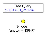
Now we may create our first simple query. We shall search for all
nodes of the type t-node (tectogrammatical nodes in
PDT 2.0) that whose attribute functor equals to
DPHR. In TrEd, the query can be created in several
ways:
Method 1: Press Insert or
 on the toolbar to create a new
selector, choose
on the toolbar to create a new
selector, choose t-nodefrom the offered list of node types and confirm with .Then press = or
 to create a new atomic
constraint, and fill
to create a new atomic
constraint, and fill functorasaand"DPHR"asbin the form (both the attribute name and its value can be selected from a list).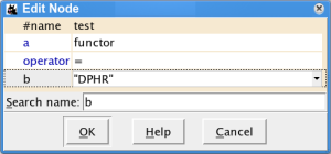
Method 2: Press e or
 to open the query text editor
and type
to open the query text editor
and type t-node [ functor='DPHR' ]
into the text field.
Method 3: Open the query text editor as above, but use helper buttons below the text field to build the text of the query: Press and select
t-node, Press , put the cursor between the brackets by clicking there or by pressing the left arrow two times, press and selectfunctorand finally press and select"DPHR".
The result in TrEd will look like this:
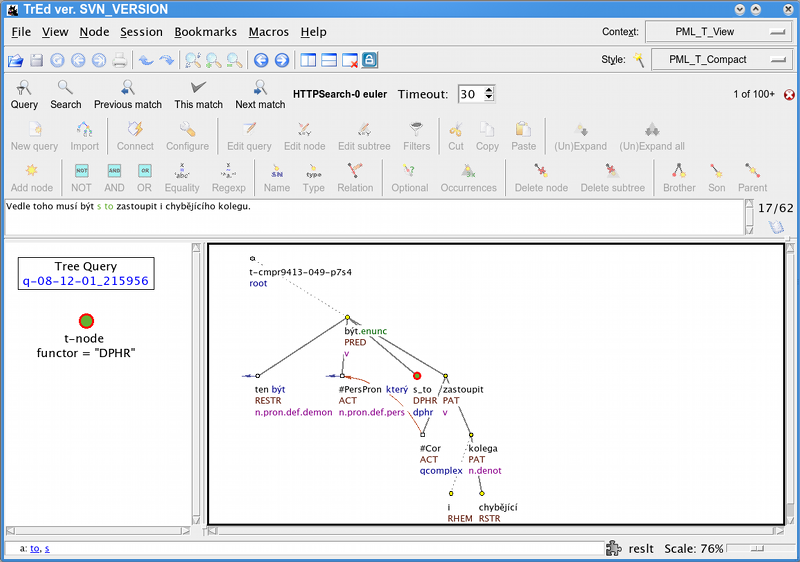
To start the search now, press Space or
![]() or
or ![]() . After a while, a window will pop up
indicating whether some results have been found, and pressing
. After a while, a window will pop up
indicating whether some results have been found, and pressing
Display will show the first result in a new view:
To see the full sentence in the text field above the
trees , click on the result view on the right. Next result can be
displayed by pressing the key n or
![]() .
.
Note
By default, the search engine returns up to 100 matches (in no
particular order), which should be more than sufficient for viewing a
few matching examples. This limit can be changed in the search engine
configuration (displayed by pressing C or
![]() , but raising this limit may slow
the search. We shall later see how to compute the number of all
matches, using output filters.
, but raising this limit may slow
the search. We shall later see how to compute the number of all
matches, using output filters.
Press p or ![]() to go back to the previous match and
press
to go back to the previous match and
press ![]() to return the current match to
view.
to return the current match to
view.
Note that the result view contains not only the matching tree but
the complete document, so it is possible to see the tree preceding or
following the currently matching tree by pressing Page
Up/ ![]() or Page
Down/
or Page
Down/ ![]() , respectively.
, respectively.
We shall now make the query more complex by adding another node to it. We shall ask for a t-node with functor "DPHR" that has a child (since DPHR t-nodes are often leaves, it may be interesting to see what children we get).
To add a new child, select the only node in our query tree and
press Insert or ![]() on the toolbar. Now a pop-up window
shows asking for a type of relation the new node to the existing node.
The default value is
on the toolbar. Now a pop-up window
shows asking for a type of relation the new node to the existing node.
The default value is child. Since this is what we
want, click . TrEd automatically assumes the
new query node to be a selector for nodes of the type
t-node, since, according to the PML schema of the
tectogrammatical layer, a t-node can only have a
t-node for its child; otherwise it would offer a list
of nodes types to choose from.
In text form, the query can be equivalently expressed as
t-node [ functor='DPHR', t-node [ ] ]
or
t-node [ functor='DPHR', child t-node [ ] ]
These forms use nesting of node selectors, the first form makes use of
the fact that the default relation of a nested selector to the selector
in which it is nested is child.
The query can also be expressed without nesting, using names, either as
t-node $a := [ functor='DPHR', child $b ];
t-node $b := [ ];
or
t-node $a := [ functor='DPHR' ];
t-node $b := [ parent $a ];
naming the two nodes
$a and $b and either indicating
that $a has a child $b or that $b
has a parent $a.
We now extend our query expression to cover also t-nodes with
functor CPHR. This can be done in three different
ways:
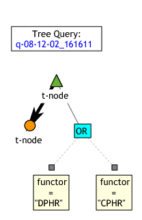
Using a disjunction:
t-node [ functor='DPHR' or functor='CPHR', t-node [ ] ]
Apart from editing the query, this can be created using the GUI e.g. in the following steps:
Select the top query node (the one with the
functor="DPHR"constraintPress h or
 to expand the constraints to
auxiliary nodes in the query tree. The result will look like
this:
to expand the constraints to
auxiliary nodes in the query tree. The result will look like
this:Select the auxiliary node representing the constraint
functor="DPHR"and press o or to create an auxiliary
ORnode above it.Select the
ORnode and press = or to create a new equality
constraint and as above, fill functorasaand"CPHR"asbin the form. Alternatively, you can select the nodefunctor="DPHR", press Ctrl+Insert or to copy it into the clipboard,
then select the
to copy it into the clipboard,
then select the ORnode and press Shift+Insert or to paste it. Then press
Enter or double-click the node or just the word
to paste it. Then press
Enter or double-click the node or just the word
"DPHR"on one of the two nodes and change"DPHR"to"CPHR".The result will look like this:
Selecting the top t-node and pressing h or
hides the auxiliary nodes, and
gives this: 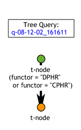
Using a regular expression:
t-node [ functor ~ '[CD]PHR', t-node [ ] ]
Symbol ~ (tilde) denotes a binary relation between
two values that is true if and only if the value on the left interpreted
as string matches the value on the right interpreted as regular
expression. The regular expression [CD]PHR is matched
by any string containing either CPHR or
DPHR as a substring. If, for example,
XDPHR were a possible functor value, we would have to
be more precise and rewrite the expression as
t-node [ functor ~ "^[CD]PHR$", t-node [ ] ]
Since ^ and $ meta-characters are
only matched by the start and end of a string, the value of
functor now must be exactly CPHR
or DPHR.
Creating a regular expression test graphically in TrEd is similar
to creating an equality test: either press ~ key or the
![]() toolbar button. Do not forget to
enclose the regular expression (field labeled
toolbar button. Do not forget to
enclose the regular expression (field labeled b in
the dialog) into apostrophes or quotes since in the PML-TQ syntax it is
just a literal string.
Using a set enumeration:
t-node [ functor in { "CPHR", "DPHR" }, t-node [ ] ]The relation in asserts that the value computed
from the expression on the left equals to a value of some of the
expressions listed in the set enumeration on the right.
The query text editor provides a button that, for attributes with a fixed set of possible values, allows the enumeration to be created by selecting the desired values from a list.
The nodes in the query can be linked by several types of
relations. The built-in relations are the structural relations (child,
parent, ancestor, descendant, sibling, same-tree-as,
same-document-as), ordering relations (depth-first-precedes,
depth-first-follows, order-precedes, order-follows). The name of a
built-in relation can optionally be followed by a pair of colons
:: in order to distinguish it from PML reference
relations described below.
The PML data model allows connecting nodes (and other data
structures) by so called PML references. In PML-TQ one can use any PML
reference as a relation by using the attribute path of an attribute
containing the reference, optionally followed by
-> (in order to prevent a collision with a
similarly named built-in or implementation specific relations). For
example, in PDT 2.0, the nodes on the t-layer are connected to nodes
on the a-layer using a PML references in the attributes
a/lex.rf and a/aux.rf. The
following query uses the a/lex.rf PML reference as
a relation:
# t-layer dependency reversed on a-layer
a-node $A := [
 child a-node $B := [  ]
];

t-node [
  child t-node [
    a/lex.rf $A
  ],
  a/lex.rf $B
];
PML references are also used in PDT 2.0 to represent textual and
grammatical coreference links (attributes
coref_text.rf and
coref_gram.rf). For example, the following query
searches for a grammatical coreference where referring node precedes
the referred node. The query defines selectors for two
tectogrammatical nodes $referring and
$referred connected by a grammatical-coreference
link coref_gram.rf, such that the lexical
counterpart of $referred follows that of
$referring in the ordering of the a-layer (which
coincides with the ordering of the original sentence).
t-node $referring := [
 a/lex.rf a-node $referring_lex := [],
 coref_gram.rf t-node $referred := [
   a/lex.rf a-node $referred_lex := [ order-follows $referring_lex ],
 ]
]
In the last example, the two t-nodes were directly connected by
a grammatical-coreference link. If we want to look for nodes connected
by a chain of grammatical-coreference links, we can do it by using a
transitive closure of the relation coref_gram.rf,
which can be expressed in PML-TQ as
coref_gram.rf{1,}. The lower bound
1 means we are looking for chains of length at
least 1 and the absence of the upper bound means that we put no limits
on the length of the chain.
t-node $referring := [
 a/lex.rf a-node $referring_lex := [],
 coref_gram.rf{1,} t-node $referred := [
   a/lex.rf a-node $referred_lex := [ order-follows $referring_lex ],
 ]
]
In TrEd, a relation can be made transitive by specifying the minimum and/or maximum bound; this can be done e.g. by double-clicking on an existing relation arrow.
Note that in the case of a cyclic chain of PML references, the chains maximum length is the number of distinct nodes in the chain plus one (i.e. the chain is allowed to start and end on the same node, but it is not allowed to continue another round along the cycle). For example, the following query searches for a cycle in the annotation of textual coreference in the PDT 2.0 tectogrammatical annotation (indeed, there is one cycle of length 2 left there by a mistake):
t-node $t := [
 coref_gram.rf{1,} $t
]Finally, any particular implementation or installation of the
PML-TQ query engine can extend the language by defining and
implementing additional specific relations. The relations behave
syntactically as the built-in relations and must use different names
than the built-in relations (their name can be followed by a pair of
colons :: in order to distinguish them from a PML
reference relation).
The current implementation defines two relations specific for
the PDT 2.0 annotation: echild and
eparent. These relations can be used both on
tectogrammatical and analytical layer and represent the effective
dependency, rather than technical dependency represented by the
built-in relations child and
parent. Thus, they abstract from certain
constructions such as coordination and apposition as well as the
dominance of prepositions (afun="AuxP") and
connectives (afun="AuxC") on the analytical
layer.
Here are a few examples of queries using these relations:
# a semantic verb with an ACT(or) and EFF(ect)
t-node [
  gram/sempos='v',
  echild t-node [ functor='ACT' ],
  echild t-node [ functor='EFF' ],
]
# a t-node with two effective parents (common modifier of coordinated nodes)
t-node [
  eparent t-node [ ],
  eparent t-node [ ],
]
# a verb with no actant
t-node $a := [ gram/sempos='v',
  ! echild t-node [ functor in { 'ACT','PAT','ADDR','ORIG','EFF' } ]
]
# reversed effective dependency on a-layer and t-layer
# excluding numeric constructions
a-node $A := [
  m/tag !~ '^C',
  echild a-node $B := [
    m/tag !~ '^C'
  ]
];
t-node [
  a/lex.rf $B,
  echild t-node [ a/lex.rf $A ]
];
Just like PML reference relations, specific relations can be used in the transitive form by setting minimum and maximum bounds, for example:
# effective descendant
t-node [ echild{1,} t-node [ ] ]
# effective grand-grand child
t-node [ echild{2,2} t-node [ ] ]The member selector is useful for querying some types of complex-valued node attributes, e.g. lists of complex structures. Such attributes do not occur in PDT 2.0, but do occur for example in CoNLL-2009 Shared Task data when converted to PML.
Each node in CoNLL-2009 ST data can be annotated as an argument of
some other node, called predicate. The argument node carries an
attribute apreds which is a list of all predicates it
belongs to. The list consists of structures with two members: a PML
reference to the predicate node (apreds/target.rf)
and an argument label apreds/label. The set of
argument labels differs from language to language; for Czech data, the
labels correspond to tectogrammatical functors and the predicates to
effective parents.
So, each structure in the list represents one labeled semantic
relation. To be able to combine constraints on the target node
(predicate) with the label of the relation that points to it, we must
use a feature of PML-TQ called member
selectors.
The following example finds a PAT argument and its corresponding predicate:
node $arg := [
  member apreds [
    label = 'PAT',
    target.rf node $pred := [ ]
  ]
]
The intermediate member selector matches one
element of the apreds list at a time and tests its
label. If the label matches, the nested node selector for the
target.rf PML-reference relation takes action.
More details and further examples are given in the section called “Member selectors”.
Sometimes it is useful to test existence, non-existence or number of occurrences of a node related to our query. For example, to find all predicates without a subject in PDT 2.0, we could use the following query
a-node [ afun='Pred', 0x echild a-node [ afun='Sb' ] ]
The query finds an a-node with afun='Pred' that
has no effective children with afun='Sb'. This is
expressed using a selector preceded by a restriction on number of
occurrences (0x - zero times), which is called a subquery.
To create a subquery graphically in TrEd, simply create the
selector echild a-node [ afun='Sb' ] as usual and
then, with the corresponding query subtree selected, press
x or ![]() .
.
Of course, we could constrain the number of occurrences to a non-zero value, too. For example, to find all predicates that govern one subject or one object, but not both, we could use the following query:
a-node [ afun='Pred', 1x echild a-node [ afun in {'Sb','Obj'} ] ]The nodes matched by subqueries are not part of the result match (in our example, the match would consist of the predicate nodes only, the subjects or objects would not be included).
The number of occurrences of a subquery can be constrained not
only to a single number (0 in our example) but to any finite union of
bounded or partially unbounded intervals of positive integers; e.g.
0|2..4|6+x restricts the number of occurrences to
zero, two to four, or six or more, eliminating one and five. While the
plus sign stands for or more, the minus sign means
or less, as in 4-x (occurring
four or less times).
Subqueries are also created using boolean operators, such as negation:
a-node [ afun='Pred', ! echild a-node [ afun='Sb' ] ]
In this example, the selector ! echild a-node [ afun='Sb'
] is automatically turned into a (still negated) subquery with
one and more occurrences; the query becomes:
a-node [ afun='Pred', ! 1+x echild a-node [ afun='Sb' ] ]
To create this query graphically, create the selector
echild a-node [ afun='Sb' ] as usual, then select the
query node corresponding to a-node [ afun='Pred' ],
create a negation node (press ! or
![]() ) and drag the query subtree
corresponding to the subject onto the negation node.
) and drag the query subtree
corresponding to the subject onto the negation node.
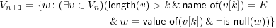
A common use of subqueries is also constraining nodes on a
descending path from one node to another. Let us for example formulate a
query searching for a descending chain of tectogrammatical nodes with
the functor RSTR (restrictive or descriptive
abdominal modification). We want the chain to satisfy the following
conditions:
The corresponding query looks like this:
t-node $N:= [
  # condition 1.
  gram/sempos ~ "^n",
  functor != "RSTR",

  # conditions 2. and 3.
  descendant{3,} t-node $R := [
    functor = "RSTR",
    # condition 4.
    0x  t-node [ functor = "RSTR" ]
  ],

  # condition 5.
  0x descendant t-node [
    !functor = "RSTR",
    descendant $R
  ],
];
Note how the condition 5. is expressed:
we say that there is no descendant of $N dominating $R whose
functor would not equal RSTR.
Thus, we have rewritten the original condition of the form
 as
as  .
.
Sometimes you want to find a good small example tree demonstrating some linguistic phenomenon. You want it to fit to a presentation slide or an article page. You can do so by putting a limit on the tree size.
Using a subquery this can be done as follows:
t-node [
  10-x same-tree-as t-node [],
  functor='DPHR', # the rest of your query
]
This selects t-nodes with functor='DPHR' in
trees with at most 10 other t-nodes. Using functions, this can be
written as
t-root [
  descendants() <= 10,
  descendant t-node [ functor='DPHR' ]
]
but note that in this case the t-root appears
as a node in the result set. To avoid it, we can write
t-node [
  functor='DPHR',
  1x ancestor t-root [ descendants() <= 10 ]
]
For treebanks that do not have a special node type for the root node, we can write e.g.:
node [
  functor='DPHR',
  1x ancestor node [
    depth() = 0, # the root
    descendants() <= 10
  ]
]PML-TQ provides a set of built-in functions that can be used in expressions constraining nodes and also in output filters. The functions can be split into the following categories:
functions returning information about the tree structure
functions related information about documents
string functions
numerical functions
group functions (applicable only in output filters)
For description of all individual functions, refer to the section called “Functions”. Here, we only give a few examples demonstrating the use of some of the functions from the first category on a few common query constructions, usually also expressible by means of subqueries. Whether it is more efficient to use functions than subqueries may depend on implementation.
# a leaf node (using functions)
t-node [ sons()=0 ]
The above query can be created graphically in TrEd by creating a
t-node selector (press Insert or
![]() on the toolbar and select a node
type (t-node in our example) from the list), then
create an equality constraint by pressing = or
on the toolbar and select a node
type (t-node in our example) from the list), then
create an equality constraint by pressing = or
![]() and fill-in
and fill-in
sons() as a and
0 as a.
Alternatively, type the query in the text form editor (opened by
pressing e or ![]() ). The function names with argument
templates can be inserted using the Functions
button in the editor.
). The function names with argument
templates can be inserted using the Functions
button in the editor.
Other queries involving functions can be created similarly.
# a leaf node (using a subquery)
t-node [ 0x child t-node [ ] ]
# right-most child
t-node [ rbrothers()=0 ]
# left-most child
t-node [ lbrothers()=0 ]
# first leaf node in a subtree of $t (using functions)
t-node $t := [
  descendant t-node [
    sons()=0,
    depth_first_order()-depth()=depth_first_order($t)-depth($t)
  ]
]
# first leaf node in a subtree of $t (using a subquery) t-node $t := [ descendant t-node $d := [ sons()=0 ], 0x descendant [ sons()=0, depth-first-precedes $d ], ]
# last leaf node in a subtree of $t
t-node $t := [
  descendant t-node [
    sons()=0,
    depth_first_order()-depth()=depth_first_order($t)+descendants($t)-1-depth($t)
  ]
]
# last leaf node in a subtree of $t (using a subquery) t-node $t := [ descendant t-node $d := [ sons()=0 ], 0x descendant [ depth-first-follows $d ], ]
Output filters are used for extracting data from the nodes matched
by the query and generating tabular output. Filters must follow the
selective part of the query and start with >>.
Filters can be chained: the first filter extracts data from the matching
nodes and all subsequent filters operate on the output from the
immediately preceding filter. Details can be found in the PML-TQ Syntax Reference and the section called “Group Functions”.
The TrEd GUI does not provide any graphical builder for
output-filter nor does it represent the filters graphically. To enter a
filter, open the entire query in the query editor (press Ctrl+E or ![]() on the toolbar), place the cursor at
the end of the query and enter the filter code. Various buttons in the
editor can be used to insert special symbols, and templates for
functions and common constructions.
on the toolbar), place the cursor at
the end of the query and enter the filter code. Various buttons in the
editor can be used to insert special symbols, and templates for
functions and common constructions.
One of the simplest filters uses the group function
count() to compute the total number of matches of the
query in the treebank:
# counting occurrences
t-node [ functor='DPHR' ]
>> count()
The group functions min(),
max(), and avg(), can be used to
compute maximum, minimum, and average values of data extracted from the
matching nodes. For example: to compute a maximum number of child nodes
of a t-node with the functor DPHR, we can use the
following:
t-node $n := [ functor='DPHR' ]
>> max(sons($n))
The following query computes maximum, minimum and average size of a tectogrammatical tree:
t-root $n := [ ]
>> descendants($n)
>> max(), min(), avg()
The above query uses two filters: the first extracts the number of
descendants from each node matched by the selector
$n, the second computes maximum, minimum and average
value from the values returned by the first filter.
The following query shows a common grouping construction using the
'for' clause. It extracts the attribute functor from
the matched nodes and for each distinct value counts the number it
occurred:
t-node $n := [ ]
>> for $n.functor
   give $1, count()
Note that $1 in the give
clause refers to the first (and only) key used in the
for clause, i.e. to
$n.functor.
By appending a sort by clause to a filter, we
may reorder the rows it produces by some of its columns. In the
following query, the output of the filter is sorted using the second
output column (the count()) in descendant order as
the primary key and the first output column (the $1
in the give clause) in the default (ascending)
order:
t-node $n := [ ]
>> for $n.functor
   give $1, count()
   sort by $2 desc, $1
The for clause can be used to create groups not
only by attribute values, but also by some of the matching nodes. For
example, in order to find out how many grammatical-coreference links can
start in one tectogrammatical node, we may use the following
query:
t-node $referring := [
  coref_gram.rf t-node $referred := [  ]
];
>>  for $referring give count()
>> max()
The selective part of the query matches every pair of
tectogrammatical nodes that are linked by a grammatical-coreference
link. The first filter groups the resulting pairs of nodes by the first
of the nodes ($referring) and outputs the number of
pairs in each group; this is the number of grammatical-coreference links
starting in the node $referring. The second filter
simply computes the maximum of the values returned by the first
filter.
The for clause partitions all input rows into
groups before any further processing and the subsequent
give clause then produces one output row for each
group, letting all group functions, such as count(),
min(), max(), etc. operate on the
particular group.
PML-TQ further supports a syntax that allows different partitions
to be defined for different group function and also let the
give clause operate on all input rows. This is done
by following the function arguments by an over
clause. Here we show an example where we use one of the ranking group
functions (row_number()) to select just a few top
ranking rows from each group. Please refer to the section called “Group functions explained” for more examples.
In the following query we extract the syntactic label
(afun) and the part of speech (the first position of
the morphological tag) from every node on the analytical
(morphosyntactical) layer of PDT 2.0. Then we apply further filters to
output in order to obtain the three most frequent parts of speech for
each afun. If several parts of speech occur the same
number of times for a given afun, we sample those three that come first
alphabetically.
a-node $a:= [ ]
>> $a.afun, substr($a.m/tag,0,1)  # get afun and part of speech (POS)
>> for $1,$2 give $1, $2, count() # count occurrences of POS for each afun
>> $1, $2, row_number(over $1 sort by $3 desc, $2) # get the rank of each POS over the afun
   sort by $1, $3
>> filter $3 <= 3
>> $1, $2, $3
A complete graphical user interface for PML-TQ is available as an extension to the tree editor TrEd and provides the following features:
interactive graphical query builder
intelligent text query editor
client interface for remote PML-TQ search server
built-in sequential search engine for local files
visualization of resulting trees and documents
multiple views for queries spanning over several layers or trees
query history (queries stored in a local file)
To use this interface, start by downloading and installing the tree editor TrEd from http://ufal.mff.cuni.cz/~pajas/tred/. The PML-TQ interface is available as an extension called PML Tree Query Interface for TrEd (pmltq) which can be either selected during installation of TrEd (on Windows) or from TrEd as follows:
Start TrEd
Select → from the main menu
In the extension manager dialog press button (connection to the Internet is required at this point).
In the list of available extensions locate an extension titled PML Tree Query Interface for TrEd (pmltq) and check the checkbutton beside it.
If you intend to query some treebanks for which a specific TrEd extension is provided, such as Prague Dependency Treebank 2.0, Penn Treebank, Penn Arabic Treebank, Tiger Corpus, CoNLL 2009 Shared Task data set etc, check those extensions as well.
Press the button, wait for the installation to complete and close the extension manager with the button.
See the section called “Tutorial” for a quick introduction to the query interface.
The PML-TQ search servers provide a client interface in the form of a web application that can be accessed by any web browser capable of combining JavaScript, CSS, and SVG (Scalable Vector Graphics). At the time of writing this tutorial, the best choice is the Opera browser, followed by Google Chrome, Firefox, and Safari (please avoid Microsoft Internet Explorer because it lacks native SVG support).
Unlike the TrEd interface, this interface does not require any installation, but lacks some features such as graphical query builder and graphical representation of the query (the queries must be entered in the text form), and of course does not support querying local files. The history of past queries is available for queries run on the particular PML-TQ search service.
For a quick introduction to the query language, see the section called “Tutorial” (only the text version of the queries is applicable).
To start using the web interface, simply open the PML-TQ server URL in a web browser, enter your query and press .
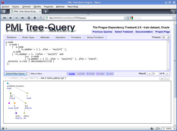
Results of queries with output filters are displayed as an HTML
table, queries without filters are rendered using SVG with the matching
nodes highlighted by colours. A simple toolbar is displayed above the
tree, with buttons for scaling the SVG image and displaying next, Nth,
or previous match. For each matching node a button in a corresponding
color is created above the displayed tree; by pressing the button, the
tree containing the particular node can be displayed, which is useful
for queries whose match can span across several trees or several
annotation layers (see Figure 1, “The Opera browser displaying a query and a result tree” Below the toolbar,
the file name, tree number, total number of trees in the file and the
sentence (or other kind of textual representation) of the tree is
displayed. The < and > links
preceding the file name can be used to display neighboring trees from
the same document.
PML-TQ comes with a command-line client utility called
pmltq. The tool can be used to perform queries
remotely (by connecting to a remote PML-TQ search engine) or locally
(using one of the tools that come with the TrEd toolkit:
btred, ntred, and
jtred).
Currently this client is able to produces plain-text output only, so it is best used in connection with queries that provide output filters.
TODO: general usage yet to be documented. Run
pmltq --help
to display information about the program command-line options and usage.
Basic examples, syntax reference.
Selectors
| Selector for nodes of a given type (list of types depends on the treebank) |
| Named selector (can be referred to as
|
Node relationships
(Please note that relations order-follows and order-precedes are implemented differently in the local search and in the server-based search. The description below aplies to the local search implementation; for the server-based search, the relations behave the opposite way.)
|
|
|
|
|
|
|
|
|
|
|
|
|
|
|
|
|
|
|
|
|
|
|
|
|
|
|
|
|
|
|
|
|
|
|
|
|
|
|
|
|
|
|
|
|
|
|
|
|
|
Logical expressions
Value comparison
Arithmetical and string operators
Subquery and number of occurrences
Functions
Output filters
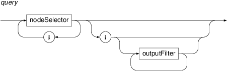
- query
PML-TQ query consists of one or more node selectors separated by semicolon followed, optionally, by a list of output filters.
- nodeSelector
Defines a node selector that selects all nodes of type
typethat satisfy given constraints. The selector can optionally be associated with a variable for reference from other nodes.The intended way to translate the selector syntax to English is to read “node of type
TYPEthat hasconstraint-1, hasconstraint-2, ... and hasconstraint-N”A selector can be used as a constraint of some other selector (i.e. it can be nested). If not preceded by a name of a relation, it selects among child nodes of the node matched by the containing selector; if preceded by a name of a relation, it selects among nodes that are in the particular relation to the node matched by the containing selector.
For example, the query
a-node $x := [ descendant
            a-node [ afun=$x.afun ] ]
reads in English as “ Find a node$xof type a-node that has a descendant node of type a-node that hasafunequal toafunof$x. ” Over PDT 2.0 data it selects all analytical nodes whose subtree contains an analytical node with the same value of the attributeafun(the query returns pairs of nodes with the described relationship).- variable
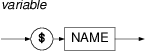
Variables are used to name node selectors and refer to them from other parts of the query. Variable starts with a '
$' (dollar) character and is followed by a NAME consisting of alphabetical character or underscore and zero or more alphanumerical characters or underscores. For example,$foo_02or$xare valid variable names, while$23is not.- constraints
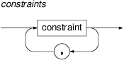
One or more constraints.
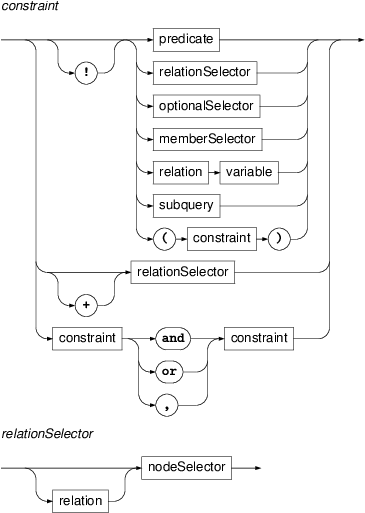
- constraint
The logical operators have the following precedence (in decreasing order): '
!', 'and', 'or', ','; except for having the lowest precedence, comma (,) has the semantics ofand. A constraint is either a binary test predicate (=,!=,~,!~,<,<=,>etc.) on expressions (terms), a node selector, member selector, subquery, a reference to a named node selector (indicating that a node matched by referred selector must be in the corresponding relation to the node matched by the current selector), or a logical combination of any of these. However, a node selector used in a complex logical expression is treated as a subquery with at least one occurrence.The intended way of reading a constraint aloud in English in the context of a node selector is to precede it with the word “has”.
By default only distinct nodes are matched by the query. If however the relationSelector is denoted by
+the matched nodes do not have to be disjoint from the other nodes matched by the query. This is usefull for printing the whole sentences like in the following example:a-node [ afun = 'AuxV', ancestor a-root $r := [ + descendant a-node $a := [ ] ] ]; >> for $r.id,$a.m/form,$a.ord give $1,$2,$3 >> give distinct concat($2, ' ' over $1 sort by $3)This example prints the sentences with an auxiliary verb (afun='AuxV'). The first matched node won't be among descendants of the root node unless the selector is denoted by
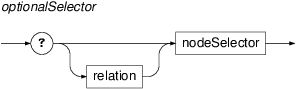
+.- optionalSelector
If a nested node selector is preceded by a question mark, it is optional. This means, that if no node matches this selector, the selector is assumed to match the same node as its containing selector and all selectors or subqueries directly nested in the optional selector are then evaluated as if they were nested in the containing selector. For example,
a-node $a := [ afun='Sb', ? a-node $b:= [ afun='AuxC', a-node $c
            := [ afun='Obj'] ] ]
with $b optional, matches either a descending chain of three a-nodes 'Sb->AuxC->Obj' (the optional selector $b matching the middle node) or just the pair 'Sb->Obj', in which case both $a and $b are identified with the 'Sb' (the constraintafun='AuxC') on $b is disregarded), but it does not, for instance, match a descending chain 'Sb->ExD->Obj'.- member selector
Member selector can be used to match complex values in node attributes of alternative, list, or sequence type. The selected value is then treated almost as a node. Although we do not indicate it explicitly in the syntax, member selectors cannot nest node selectors via tree-structure or ordering relations.
Member selectors are described in detail more in the section called “Member selectors”.
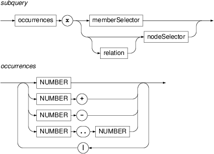
- subquery
Subquery is a nested selector with a constraint on the number of occurrences of the matching nodes (with respect to a fixed match of the containing selector). For example,
3xspecifies that the subquery must match exactly three times,3+xspecifies that it must match at least three times,3-xspecifies it must match at most three times, and3-10xspecifies that it must match at least three times and at most ten times.Note
Node selectors that belong to a subquery cannot be referred to by name from outside the subquery (outer scope).
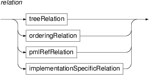
- relation
PML-TQ has the following types of relation:
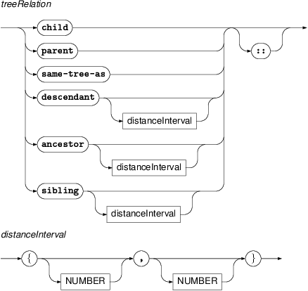
- tree relations
These are child, parent, descendant, ancestor, and sibling. The last three can be followed by a distance interval of the forms
{min,max}, or{,max}, or{min,}whereminandmaxare integers withminless than or equal tomax. These values must be positive for the relationsdescendantandancestor. For thesiblingrelation, negative distance bound values range over preceding siblings and positive bound values range over following siblings.For example, in the query
t-node $a := [ sibling{-1,2} t-node $b := [ ] ]the node
$bcan be either the immediately preceding sibling of$aor one of the two siblings immediately following$a.In the query
t-node $a := [ descendant{3,} t-node $b := [ ] ]$bmatches a descendant of$asuch that there are at least two nodes on the path from $a to $b strictly between $a to $b.- ordering relations
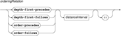
Relations
depth-first-precedesanddepth-first-followsconstraint mutual position of two nodes in the canonical depth first ordering of the tree.Relations
order-precedes,order-followsare only available for treebanks with explicit total ordering on the trees (typically dependency treebanks).These relations can be followed by a distance interval of the forms
{min,max}, or{,max}, or{min,}whereminandmaxare (possibly negative) integers, withminless than or equal tomax.For example, in
t-node $a := [ depth-first-precedes t-node $b := [ order-precedes $a ] ]
$amatches a node that precedes$bin the depth-first order but follows$bin the total ordering of the tree; thus, for instance,$bcan be a descendant of$athat precedes$a.In the following query,
$amust immediately precede$bin the total ordering of the tree:t-node $a := [ order-precedes{,1} t-node $b := [ ] ]Conversely, in
t-node $a := [ order-precedes{2,} t-node $b := [ ] ]$aprecedes$b, but there must be at least one other node between the nodes$aand$b. The queryt-node $a := [ order-precedes{1,2} t-node $b := [ ] ]allows at most one node between
$aand$bin the total ordering of the tree.Negative distance bound extends the relation in the opposite direction. For example, in this query:
t-node $a := [ order-precedes{-1,1} t-node $b := [ ] ]$aeither immediately precedes$bor immediately follows$b.- relations based on PML-references
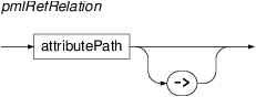
These relations represent ID-based references. They are derived from attributes declared in the specific PML schema of the treebank as PML references and represent the relation from a referring node (the one containing the reference) to the referenced node (the one whose ID the reference contains).
The name of the relation is an attribute path to a PML reference (declared in the PML schema as
<cdata format="PMLREF"/>).For example, nodes of the type
t-nodein PDT 2.0 are structures declares as follows:<type name="t-node.type"> <structure role="#NODE" name="t-node"> ... <member name="a"> <structure> <member name="lex.rf"> <cdata format="PMLREF"/> </member> <member name="aux.rf"> <list ordered="0"> <cdata format="PMLREF"/> </list> </member> </structure> </member> ... </structure> </type>So, for a
t-node, the attribute pathsa/lex.rfanda/aux.rfrefer to PML references. They represent a pointer to a lexical counterpart node on the analytical layer, and zero or more pointers to related auxiliary nodes on the analytical layer (prepositions, conjunctions, auxiliary verbs, etc.). We can thus use these relations as follows:t-node $t:= [ a/lex.rf a-node $a:= [ afun='Sb' ], a/aux.rf a-node $x:= [ afun = 'AuxP' ] ]
The query locates a
t-node$twhose lexical counterpart on the analytical layer is the node$bwithafun='Sb'and that contains at least one pointer to an auxiliary node$xwithafun='AuxP'(a preposition).Since the names of node attributes may be in collision with other types of relations, we may force interpreting a relation as a
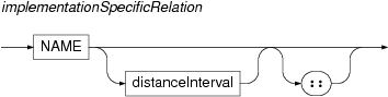
pmlRefRelationby following it by the characters->.- implementation specific relations
An implementation can choose to provide further set of relations provided that their names are not in collision with the tree relations and ordering relations.
For example, the standard implementation of PML-TQ defines relations
echildandeparentfor the PDT 2.0 treebank to represent so called effective-parent and effective-child relations.These relations can be optionally followed by an interval bounding the number of transitive applications of the relation. It can be of the forms
{min,max}, or{,max}, or{min,}whereminandmaxare positive integers, withminless than or equal tomax.For example,
eparent{1,}is a transitive closure of theeparentrelation (i.e.\ effective ancestor). Similarly, int-node $a:=[ echild{1,2} t-node $b:=[] ]the node
$amust be an effective parent or effective parent of an effective grand parent of$b. The queriest-node $a:=[ echild t-node $b:=[] ]
and
t-node $a:=[ echild{1,1} t-node $b:=[] ]are equivalent.
All relation names except for PML-reference relations can be followed by two colons in cases that could lead to syntactical ambiguity (e.g. if they can be confused with node types). PML-reference relations can be followed by an arrow (a dash and greater-than characters) to avoid confusion with other relations, node types, or keywords.
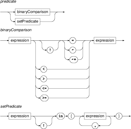
- predicate
A predicate is either a binary comparison of two expressions (terms) or a set membership predicate applied to a term and a set specified as an enumeration of other terms.
The binary comparison consists of two expressions and a binary relation. The relations
~and~*perform case-sensitive and case-insensitive regular expression matching, respectively. The expression on the right must evaluate to a regular expression. For exampleafun ~ '^(Sb|Aux.*)$'is true if the value of the attributeafunof the current node selector either equals to the stringSbor starts with the stringAux.Set predicate consists of a expression, the operator
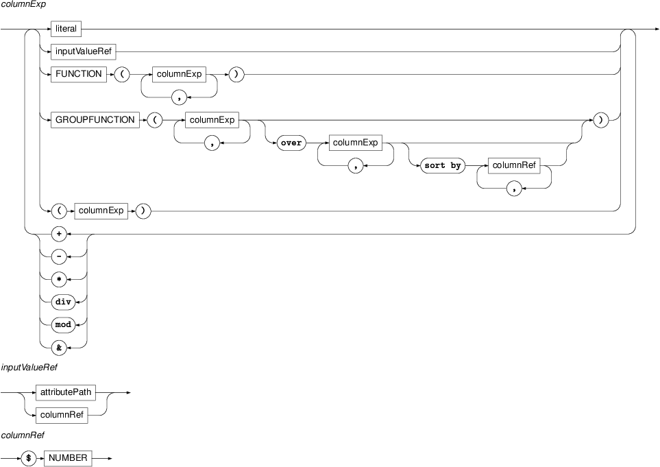
inand a comma-separated list of expressions enclosed in braces. It is true if the value computed from the expression on the left equals some of the values computed from the expressions on the right of the operator.- expression
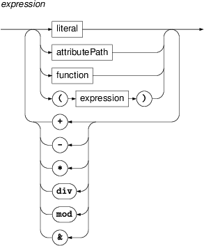
Expressions are either literals (strings, integer of floating point numbers), attribute paths, or functions, or any combination of these obtain by application of the binary string-concatenation operator ('&') or the usual arithmetical operations for addition ('+'), subtraction ('-'), multiplication ('*'), division ('div') and modulo ('mod'). Brackets can be used in the usual manner for grouping sub-expressions.
For example,
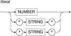
afun & "." &
            substr(m/tag,0,2)
is an expression returning a concatenation of the value of the attributeafun, a dot and the first two characters from the value of the attributem/tag.- literal
A literal is either a number in the decimal notation (integer or floating point, e.g.
231or-1.0032) or a string of characters enclosed in either"or'. Backslash character\is used as an escape character, for example to insert a quote or apostrophe.For example:
"Peter's"and'Peter\'s'are both literals representing the stringPeter's. Similarly,'\\\"\'\n\r\1'and"\\\"\'\n\r\1"are literals representing the five-character string\"'nr1. (Note that\nis not currently used for the new-line characters as in many other dialects; this however, may change in a future version so it is adviced to avoid escaping characters other than quote and apostrophe).- attributePath
An attribute path refers to a value of an attribute of a treebank node matched by a certain selector. If the path starts with a variable followed by a '.' (dot) character, then the it refers to an attribute of the node matched by the selector associated with the variable. Otherwise it refers to the node matched by the current selector (i.e. the one within whose constraints it occurs).
In the simplest form, attribute path is just a name of an attribute, e.g.
functor. However, some node attributes may have complex values, i.e. structures with attributes of their own. In such case one forms a slash-delimited attribute path leading from the node to some nested atomic value. Each component of the path (step) is either a- name
specifying a member in a structure or any element of the given name in a sequence
- the string
'content()' used for obtaining the content of a container
- index
(
[)n] specifying
n-th element in an ordered list- name followed by an index
(
foo[n] specifying
n-th element of a given name (foo) in a sequence- name preceded by an index
(
[)n]foo specifying
n-th element in a sequence and asserting that then-th element name is as given (foo)
If a partial attribute path returns an object of a list type, the next step in the path can either be an index or can be omitted (in which case any list member matches); if it returns a sequence, the next step must be an element name optionally followed or preceded by an index. If it is a structure or container, the next step must be a name of an attribute; if it returns an alternative or an unordered list, the next step must be a valid step for the members of the alternative/list; if it returns an atomic value, there must be no further step.
For example
gram/semposselects the attributesemposof a structure stored in the attributegramof the node matched by the current selector. The patha/[1]/bmay select an attribute b of a structure stored in the 2nd member of an ordered list stored in the attributea; the patha/bselects the attribute b of any member of the lista.If some part of an attribute path leads to an alternative, list, or sequence, the path may match multiple values. Assume
Ris some predicate containing such an attribute path in some of its expressions. If attribute path is preceded by the*character (a primitive universal quantifier), then the predicate is true if and only if it is true for every value matched by the attribute path. If attribute path is not preceded by*, then an existential quantifier is assumed: the predicate is true if and only if there exists a value matched by the attribute path for which the predicate is true. If the predicate contains more such attribute paths, the quantifiers (universal and implicit existential) are applied in the same order in which the attribute paths occur in the predicate. See the section called “Primitive quantifiers” for details.Example:
a-node $p:= [ child a-node [ afun=$p.afun, afun~'^Aux' ] ]
The above query selects a node and its child node (both of type
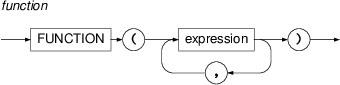
a-node) that have the same value of the attributeafunand the value starts with the substringAux.- function
Functions are written as function name followed by a comma-separated list of its arguments in brackets. The functions currently supported by PML-TQ are listed in Section the section called “Functions” :
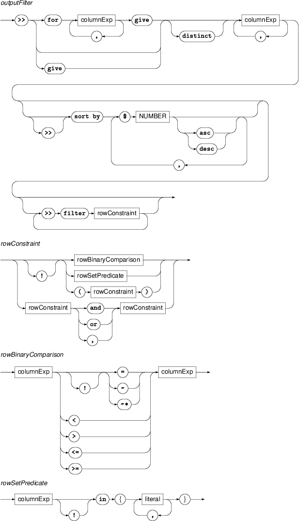
- outputFilter
An output filter transforms its input (the result of the selective part of the query or the output of the previous filter) into a table of values arranged into columns computed according to the filter specification.
The simplest form of a filter consists of a comma-separated list of expressions, each of which computes a column value in an output row from either the values of (some) column of the input row (output from the previous filter) or, in case of the first filter, the attributes of nodes matched by the selective part of the query. For example:
>> $x.m/tag, depth($y)
>> 'found ' & $1 & ' at depth ' & $2
defines two output filters: the first returns a table whose rows correspond directly to the matches of the query's selective part. Its first column contains the value of the attribute
m/tagof the node matched by the node selector$xand the second column is the depth of the node matched by the node selector$y. The second output filter produces a table with just one column with values of the formfound, whereXat depthYXandYrepresent the two columns from the preceding filter.The column expressions can also use group functions that do not specify partitioning (using an
overclause) and therefore range over the whole input table. In that case, all column expressions must result in constant values and the filter will produce a single row.For example,
>>min($1), max($1), avg($1)
is an output filter that computes the minimum, maximum and average form the values in the first column of the preceding filter (and returns a table with exactly one row having these three values in its three columns).
Each filter may be followed by a
>> sort
            by
clause which specifies the order of rows in the resulting table. The clause is followed by a comma-separated list of column references. They refer to the columns of the table produced by this filter and are used to compute the primary, secondary, tertiary,… etc. sorting key. Each column reference can be followed by the wordascordescto enforce ascendant (default) or descendant ordering on the corresponding column.The filter may optionally be preceded by a
forclause that partitions the input rows into groups according to given keys and produces one output row for each group; any group function occurring in the output column expression will range over the current group.The
forclause consists of a set of column expressions used to compute a vector of values from each input row. This vector serves as a key by which the input rows are partitioned into groups. Thegiveclause now produces one output row for each group. Note that the column references occurring in thegiveclause are interpreted as references to the columns of the key vector, except for the case of column references occurring in arguments of group functions (that do not declare its own partitioning using anoverclause), which refer to the columns of the input rows within the current group.For example:
a-node $a:= [ child a-node $b := [] ];
>> for $a.afun, $b.afun
give $1, $2, count()
sort by $3 desc
is a query whose selective part returns pairs of a-nodes in the parent-child relationship. The output filter first computes a key, in this case a vector of two of values: the attribute
afunof the parent and the child. Then it groups the results according to this key and for each group returns a row consisting of three values: the two columns from the key vector ($1, $2and the number of elements in the corresponding group (count()). Thesort byclause reorders this output by the third column in descendant order. As a result we get the frequency table of co-occurrence ofafunattribute values on an edge in the treebank with the most frequentafunpairs first, which may look like this:Atr Atr 87306 AuxP Adv 56344 Sb Atr 56269 Obj Atr 51908 Adv Atr 48741 Pred Sb 44963 Pred AuxP 39125 Pred Obj 31744 AuxP Atr 31227 Coord Atr 30569 Coord Pred 24739 Pred Adv 24196 ...
A filter can further be followed by one or more
>> filterclauses which drop certain output rows, leaving only those rows that satisfy a specific constraint. For example, the following querya-node $n:= [ ] # Filter 1 >> give lower($n.m/form) >> filter $1 ~ '^[a-z]' # Filter 2 >> for $1 give $1,count() >> filter $2 >= 1000 # Filter 3 >> give $1,$2 sort by $2 desc
retrieves a list frequent word forms from a treebank. The selective part returns each node
$nof the typea-node. For each such node, filter 1 retrieves its lowercase word form from the attributem/formand drops those forms that do not start with a letter. Filter 2 groups the rows with the same form and counts the number of rows in each group, producing a table with two columns: a form and number of its occurrences; due to the grouping, the first column now contains only unique values. Thefilterclause of Filter 2 prunes this table, preserving only rows where the number of occurrences is at least 1000. Finally, filter 3 copies both input columns and orders the table by its second column, in the decreasing order, so that the most frequent forms appear on top.- columnExp
Column expressions are expressions that additionally allow group functions and column references of the form
$whereNNThe exact rules on usage of group functions and column references in column expressions are detailed in the description of output filters above.
![nodeSelector : TYPE (variable ':=' )? \\ '[' constraints? ']' ;](rail_nodeSelector.png)
![memberSelector : 'member' attributePath (variable ':=' )? \\ '[' constraints? ']'](rail_memberSelector.png)
![attributePath : '*'? (variable '.' )? (XMLNAME | 'content()' | index | elementIndex ) + '/' ; index : '[' NUMBER ']'; elementIndex : XMLNAME index | index XMLNAME;](rail_attributePath.png)
Nodes in PML are usually attribute-value structures with values that can be of either atomic PML data types (integers, strings, etc.) or complex PML data types (structures, lists, alternatives, sequences, containers). This means that to get to an atomic value stored within a node we sometimes have to travel through several nested complex data structures, starting from the top-level structure which is the node itself. PML-TQ uses attribute paths to describe the route of such a travel.
The syntax of an attribute path is described by the attributePath production of the PML-TQ grammar.
In this section we define how attribute paths are evaluated.
(Note: complex queries over nested attribute values can be performed by
combining attribute paths with the member selector,
see the section called “Member selectors”.)
An attribute path consists of a sequence of steps separated by
slashes. This sequence can be optionally preceded by a primitive
quantifier the semantics of which is described later in the section called “Primitive quantifiers”. Each step is either a name, the string
'content()', an index, or an element index.
Let P be an attribute path consisting of steps S1,…,Sm (m>0). The result of evaluation of P on a node N is a set VN,P of atomic values (integers, floats, or character strings). The evaluation proceeds by evaluating the steps from 1 to m; the evaluation of the step Sn (1≤n≤m) takes as input a set of values Vn and results in a set of values Vn+1. For each n (1≤n≤m+1), all values in Vn are of equal data type (which, if P is a valid attribute path for N, is complex for n≤m and atomic for n=m+1).
The evaluation is initialized with a set V1={N} whose only element is the node N, which is either a structure or a container. The result of the evaluation if the set VN,p=Vm+1.
Let Vn be given. We now describe the evaluation based on the syntactic type of the n-th step Sn and the data type of values in Vn. Let tn denote the type of the values in Vn.
If tn is an atomic type (and there is an n-th step), the query compiler reports an error and fails.
If tn is a structure or container type and Sn is a name of a valid member for tn (according to the declaration of tn in the corresponding PML schema) then for every element of Vn, Vn+1 contains the value of its member Sn, provided the value is non-null; i.e.
If the step Sn is '
content()' and tn is a container type with non-void content (i.e. the container has some content type declared in the PML schema), Vn+1 consists of the content value of each element of Vn, i.e.If Sn is anything else, the query compiler reports and error and fails.
If tn is an ordered list and Sn is an index of the form
[k], where k is a non-negative integer number, then Vn+1 consists of the (k+1)-th value (v[k]) of each list in Vn whose length is at least k+1, i.e.If tn is a list or an alternative, and Sn is any step except for the case covered above (where tn was an ordered list and Sn an index), let V'n consist of all non-null values that occur in some list or alternative from Vn, i.e.
Then Vn+1 is obtained by applying the step Sn on the set V'n instead according to these rules.
If tn is a sequence type and Sn is an element name E valid for the sequence type tn, then Vn+1 consists of all non-null values of elements with a given name occurring in some sequence from Vn, i.e.
If Sn is of the form '
E[k]', where E is a valid element name for tn and k is a non-negative integer number, then for each sequence in Vn the (k+1)-st occurrence of element named E (if exists) is taken and the element's value, if non-null, is added to Vn+1. Formally,If Sn is of the form '
[k]E', where E is a valid element name for tn and k is a non-negative integer number, then for each sequence in Vn of length at least k+1 the (k+1)-st element is taken and if its name is E and its value is non-null, the value is added to Vn+1. Formally,


As described above, evaluation of an attribute path on some node may result in a set of values (usually empty or containing one element, but if lists, alternatives or sequences are on the path, the set can be of arbitrary finite cardinality). In this section we define how the truth value of a predicate involving attribute paths is evaluated. We start with the formal definition and then demonstrate it on a few examples.
Definition. Let R be a predicate and let
p1,…,pn
be an enumeration of all occurrences of attribute paths in expressions
(terms) contained in R in the order of
occurrence and let N1,…,Nn
be the nodes to which the attribute paths relate. Let for i (1≤i≤n), Qi denote the universal
quantifier  if pi starts with a '*' and
  otherwise. Let Vi denote the set VNi,pi
of atomic values obtained by evaluating the attribute paths pi on the node Ni. Then the truth value
of the predicate R for this assignment is
that of the formula
otherwise. Let Vi denote the set VNi,pi
of atomic values obtained by evaluating the attribute paths pi on the node Ni. Then the truth value
of the predicate R for this assignment is
that of the formula  where R' is an atomic
formula obtained from R by replacing the
attribute paths p1,…,pn
by variables x1,…,xn.
(Note that each of the variables has exactly one occurrence in R'.)
where R' is an atomic
formula obtained from R by replacing the
attribute paths p1,…,pn
by variables x1,…,xn.
(Note that each of the variables has exactly one occurrence in R'.)
Now let us demonstrate the definition on some examples. Let R be the predicate
*a != b/c + *$n.d/e/f
in the query
z-node $n := [ child z-node $m := [ *a != b/c + *$n.d/e/f ] ]
where z-node is some node type, and
a b/c, d/e/f
are valid attribute paths for nodes of this type. Let N and M be nodes from
the searched data assigned to the selectors $n and
$m.
Let's assume that the attribute a is a list of
numbers and that VN,a is the set of all
values of the attribute a for the node N. Similarly, let VM,b/c be the set of all
values of the attribute path b/c evaluated on the
node M and VN,d/e/f the set of all
values of the attribute path d/e/f evaluated on the
node N.
The truth value of the predicate R is obtained by evaluating the following formula:

Thus, the query matches the nodes A, B if and only if
B is a child of A and the above formula holds. Note that since the
attribute paths *a and *$a.d/e/f
start with the character '*' (called a primitive
universal quantifier) the corresponding variables x and z in the formula
(1) are universally quantified, whereas
y, corresponding to b/c
is quantified existentially. Note also, that the order of the
quantifiers in the formula (1) preserves the
order of the occurrence of the corresponding attribute paths in R.
If we had instead written
! *a = b/c + *$n.d/e/f
moving the negation (!) out of the predicate, the
resulting formula would be completely different:

and equivalent to

Let us give some more practical examples. Assume nodes of the type
p-node have an attribute functions
that is an unordered list or an alternative of string values. Let us
consider the following constraints and the translations to formulae
(assuming VN is the
set of values of the functions for a given p-node
N):
functions = functionsasserts that the listfunctionson N is non-empty, since the constraint translates to the formula which is equivalent to
 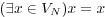 and to
  .
.functions != functionsasserts that the listfunctionson N contains (at least) two distinct strings, since it translates to .
.!functions = functionsmeans that the listfunctionson N is empty, since it is a negation offunctions=functions.*functions = *functionsasserts that the listfunctionson N contains at most one unique value because it translates to , which is satisfied if the set VN is either empty or
contains exactly one element.
, which is satisfied if the set VN is either empty or
contains exactly one element.*functions = functionsis always satisfied, because it translates to .
.functions = *functionsasserts that the listfunctionscontains exactly one unique value, since it translates to .
.*functions != functionsasserts that the listfunctionsis either empty or contains at least two unique value, since it translates to .
.functions != *functionstranslates to , which is never satisfied (since x=x).
While primitive quantifiers allow one to quantify over atomic
values on a complete attribute path, something it is useful to quantify
over elements on some partial attribute paths while specifying
conditions on the quantified element. This can be done using the
relation member, which allows us to access data
structures stored in node's attributes almost as if they were regular
nodes.
For example: assume each node contains an annotation of the
bridging anaphora. This can be represented by an attribute called
bridging that is a list of structures with two
members, informal-type (a string value for the type
of the anaphora) and target.rf (a PML reference to
the anaphora referred node). So, each element of the
bridging list represents a labeled link to another
node. We might want to ask for nodes with
functor="ACT" that are pointed to from the current
node by a pointer with a specific informal-type, say
"CONTRAST".
The following query will not work
t-node $n := [
  bridging/informal-type = "CONTRAST",
  bridging/target-node.rf t-node [ functor="ACT" ]
]
The problem with this query is that
bridging attribute contains a list and constraints on
its values are independent. So, $n can still match a
node whose bridging attribute is a list consisting of
two list members, one that points to an ACTor but whose
informal-label is not "CONTRAST",
and one with informal-label="CONTRAST" but pointing
somewhere else.
In order to be able to say that these list members are the same,
we have to use the member selector:
t-node $n:= [
  member bridging [
    informal-type = "CONTRAST",
    target-node.rf t-node [ functor="ACT" ]
  ]
]
This query says that one of the values matched by the attribute
path bridging (i.e. one of the members of the list
contained in the attribute bridging of the node
matched by $a) has
informal-type="CONTRAST" and points to a
t-node with functor="ACT". Thus,
member selector works as an existential
quantification over values of a list or alt attribute. We can also use
member selector for sequence attributes, but the
attribute path that follows the member keyword must
specify a particular element name in the last step. For example, if
bridging was not a list but a sequence of elements
named e.g. terminal, non-terminal,
we must use either
member bridging/terminal [...]
to quantify over all terminals in the bridging
sequence or
member bridging/non-terminal [...]
to quantify over all non-terminals in the bridging
sequence.
Of course, we can use member selectors within
member selectors and (as we have seen), we can use
PML-reference relations within member selectors. But
since the objects represented by the member selector
are not a regular nodes one cannot use the tree-structure selectors such
as child or parent within
member selectors.
A member selector can be used for a subquery,
i.e. prefixed by an occurrence clause or used in boolean expressions. In
particular, negated or zero-times occurring member
selector with negated constraints can be used to formulate universal
quantification over values of a list, alt, or sequence.
PML-TQ supports group functions in the output filters. These functions compute its value based on a group of input rows, not just the current row. For example, one can use them to compute a sum or maximum over a group of input rows, or a rank of the current input row in some particular ordering of the group of input rows it belongs to.
A filter can specify grouping of input rows in the following ways:
Considering all input rows as one group.
In this case case the filter produces exactly one output row whose columns are either constant or computed by applying a group function.
Examples of such filters are
>> count()
computing just the count of all input rows, or
>> concat($1), sum($2)/count(), max($2)-min($2)
computing a row consisting of three columns: the first one concatenating all values in column 1 of the input from the preceding filter, the second computing an average value of column 2 of the input (which we could also write as
avg($2)), the third the difference between maximum and minimum value column 2 of the input.Partitioning input rows into groups and evaluating group functions over each group.
This method allows one to define a partition on the input rows into groups that share some key value and then operate on each of these groups individually, producing one output row per partition group.
In the first step, the filter computes a vector of values from each input row, called a key, and puts all rows that produce the same key to one group. The filter then produces for each group one output row, computed based on the columns of the group key and group functions ranging over the group.
For example, consider the following query:
t-root $r:= [
  descendant t-node $n []
]
>> $r.id, depth($n)
>> for $1 give max($2)
>> for $1 give $1, count() sort by $2 desc
The main part of the query returns all pairs of nodes
($r,$n)where $r is a root node and $n is any of its descendants. For all such occurrences, the first filter produces a row with two columns: the (unique) ID of$rand the depth of the node$nin the tree.The second filter takes the first column of its input row (i.e. the
ID) as the key and groups the input row by this key; this results in as many groups as there were unique root nodes in the matching set and each group consists of the input rows that belong to one root. This is done by thefor $1clause. Thegive max($2)clause says that for each group, we want to produce an output row with a single column whose value is calculated as the maximum of the values in column 2 of the input filter, i.e. maximum of depths of the nodes$nfor the given root$r. This is basically the depth of the tree rooted in$r.Finally, the third filter computes a distribution of tree depths. It's input are depths of individual trees. It groups the input rows according to their first and only column (the depth). Since there is just one input column, the key vector here is the whole input row; so all rows within each group are identical. For each group, the filter counts number of rows in it and outputs a row whose first column is the first column of the group key (in our case the tree depth) and the second is the count (number of trees of the particular depth). Finally, the
sort by $2
            desc
clause orders the output table by the 2nd column in the descending order.Note that there are two types of column references in the
give...clause. Those that occur within a grouping function (such as$2inmax($2)) refer to columns of the rows in the current group. Those that occur outside a group function, (such as$1in$1,count()) refer to columns of the key vector of the current group (so it is guaranteed that this value is constant over all rows in each group).On-line grouping within group functions.
PML-TQ also allows group functions to be computed over some group of input rows without actually partitioning the input, i.e. without reducing the number of output rows to one per group. Using this method, each group function can specify its own way of grouping and ordering of the input rows. Consider this example on PDT 2.0:
t-node $a := [
  t_lemma = '#Forn',
  t-node $b := [
   functor = "FPHR"
  ]
];
>> $a.id, distinct concat($b.t_lemma, ' ' over $a sort by $b.deepord )
The selective part of the query finds t-node
$awitht_lemma='#Forn'which is a technical node governing a flat list of words in a foreign language and its child-node$bwith functorFPHR(foreign phrase), which matches any of the words.To reconstruct the foreign phrase, we need for each
$ato concatenate thet_lemmaof all corresponding$b's in the ordering of the tree (given by the attributedeepord).The input to our filter are the pairs of nodes
$aand$b. The concatenation is performed by the group functionconcat. The first argument says which value we want to extract from each input, the second argument' 'is optional and specifies a separator of the concatenated values. Theover ...clause defines partitioning into groups just as thefor ...clause; the difference is that this partitioning is particular to this group function, not to the whole filter. In fact, given an input row, the expressionconcat($b.t_lemma, ' ' over $a ...says that we want to select those input rows where$ais the same as in the current row, and for this selection concatenate the values$b.t_lemma. Thesort by...clause says that the selected rows should be ordered by$b.deepord.Unlike partitioning using the
for...clause, this type of partitioning is done within the group function, so the filter produces one output row for each input row, not just one per group. Thus, we would get the same output for each input pair($a,$b)where$ais the same; we therefore use the keyworddistinctto filter out the duplicities from the output.Thus, on the output, we get the ID of
$aand the foreign phrase its subtree represents.This type of grouping can also be combined with the
for...clause to define a partitioning on the set of groups produced by thefor...clause. In that case, the column references within aover...clause refer to the columns of the group key of thefor...clause.The clause
over allcan be used as a special variant of theover...clause creating only one group which spans over all input rows. The same effect can also be achieved using a constant key in theover...clause, e.g.over 0.
Let us consider an example that combines grouping based on
'for' and 'over'.
Let's say that for each functor A we want to know the probability that a child of a node with functor=A has functor A, B, C, D, etc. In other words, we want to compute the joint distribution of functor labels over nodes connected by an edge. This is done by the following query:
t-node $p := [  t-node $c := [  ] ];
>>  for $p.functor,$c.functor
    give $1,$2,count() div sum(count() over $1)
    sort by $1,$3 desc,$2
>> $1,$2,percnt($3,2) & '%'
The selective part select a pair of t-nodes
($p,$c) where $p governs
$c.
We first group together pairs with the same pair of functors using
for $p.functor,$c.functor. This partitions original
input rows into groups
g1,...,gn,
each determined by the unique value of the grouping key
($p.functor,$c.functor). For each group we give to
the next filter this pair of functors and the probability of the second
functor on the first one. The filter thus produces one output row for
each group. Let us see how the output row is produced for a group
gi whose key is for example
('PRED','ACT').
The first two columns are just taken from the key vector, using
$1,$2 and producing 'PRED','ACT'. The probability
that 'ACT' is governed by 'PRED' is computed using the following
expression:
count()div sum(count() over $1)

The first | |
The So, our current group
|
The filter then orders the results primarily by the functor of the
parent node, secondarily by the probability in decreasing order, and
tertiary by the functor of the child. The second filter merely applies
the expression percnt($3,2) & '%' to the 3rd
column, dividing it by 100, rounding the result to two decimal points
and appends a percent sign.
The output looks like this (without the ellipses):
ACMP    RSTR    54.37%
ACMP    PAT     10.77%
ACMP    ACT     10.34%
ACMP    APP     4.99%
...
ACT     RSTR    49.56%
ACT     PAT     9.75%
ACT     APP     8.68%
...
ADDR    RSTR    64.67%
ADDR    APP     14.74%
ADDR    PAT     4.24%
ADDR    ID      3.17%
...
ADVS    PRED    48.5%
ADVS    ACT     13.18%
ADVS    CM      9.09%
...
The query just explained can also be rewritten as follows:
t-node $p := [ t-node $c := [  ] ];
>> $p.functor,$c.functor
>> distinct $1,$2, count(over $1,$2) div count(over $1)
   sort by $1,$3 desc, $2
>> $1, $2, percnt($3,2) & '%'
Another reformulation of the query uses the group function
ratio():
t-node $p := [ echild t-node $c :=  [  ] ];
>>  for $p.functor,$c.functor
  give $1,$2,ratio(count() over $1)
  sort by $1,$3 desc
>> $1, $2, percnt($3,2) desc
Finally, we may insert filters selecting just a few (say two) best ranking rows for each functor in the first column:
t-node $p := [ echild t-node $c :=  [  ] ];
>>  for $p.functor,$c.functor
  give $1,$2,ratio(count() over $1)
  sort by $1,$3 desc
>> $1,$2,$3, row_number(over $1)
>> filter $4<=2
>> $1, $2, percnt($3,2) desc
to produce the following output (continuing after the final ellipsis):
ACMP    RSTR    54.37%
ACMP    PAT     10.77%
ACT     RSTR    49.56%
ACT     PAT     9.75%
ADDR    RSTR    64.67%
ADDR    APP     14.74%
ADVS    PRED    48.5%
ADVS    ACT     13.18%
...
- name($var?)
Return the name of a node matched by the given selector (assume current selector if used without an argument). This function only makes sense if the node is an element of a PML sequence (of trees or child nodes).
- depth($var?)
Returns the depth in the tree (counting from 0) of a node matched by a given selector. If no argument is given, the current selector is assumed.
- descendants($var?)
Returns the number of descendants of the node matched by a given selector. If no argument is given, the current selector is assumed.
- lbrothers($var?)
Returns the number of left siblings of the node matched by a given selector. If no argument is given, the current selector is assumed.
- rbrothers($var?)
Returns the number of right siblings of the node matched by a given selector. If no argument is given, the current selector is assumed.
- sons($var?)
Returns the number of child nodes of the node matched by a given selector. If no argument is given, the current selector is assumed.
- depth_first_order($var?)
Returns the depth-first order of the node matched by the given selector (counting from 0). If no argument is given, the current selector is assumed.
- file($var?)
Returns the file name of a document in which the node matched by a given (or current) selector occurs.
- tree_no($var?)
Returns index of a tree in which a the node matched by a given (or current) selector occurs, i.e. the position of the tree in its document.
- address($var?)
Returns an URL uniquely determining the node matched by a given (or current) selector. The same value can be also computed using the following expression:
file($var) & '##'
              & tree_no($var) & '.' &
              depth_first_order($var)
.
- length(string)
Returns the string length of a given expression.
- substr(string,offset,length?)
Returns a substring of a given string starting at at a given offset (first character in the string has offset 0) and spanning for a given length or to the end of the string, if length is omitted or if the original string has less than offset+length characters.
- match(string,regexp,flags?)
Returns the first substring of a given string matching a given regular expression. The optional third argument can be a string of flags modifying the behavior of the regular expression matching procedure. The following flags are supported:
- i
case insensitive match
- c
case sensitive match (default)
- n
allows the period (.) to match the newline character
- m
Treat string as multiple lines. That is, change "^" and "$" from matching the start or end of the string to matching the start or end of any line anywhere within the string.
- replace(string,substr,replacement)
Substitutes a given replacement for all (non-overlapping) occurrences of a given substring in a given string and returns the result. For example,
replace('banana ananas','ana','ANA')returnsbANAna ANAnas.- substitute(string,regexp,replacement,flags?)
Substitutes a given replacement for the first or all (non-overlapping) substrings matching a given regular expression in a given string and returns the result.
The default behavior is to replace just the first matching substring. To replace all occurrences, use the flag 'g'.
The replacement string may contain references to subexpressions of the matching regular expression (subexpressions are parts of the expressions enclosed in brackets). The string \N, where N is a digit from 1 to 9, is a reference to the N-th subexpression (counting opening brackets from the left), and is substituted in the result by the substring matched by that subexpression. For example, if the regular expression was
a(b(c))(d), then\1,\2, and\3refer to the subexpressions(b(c)),(c), and(d), respectively.Note: in PML-TQ string literals, backslash (
\) is used as an escaping character, therfore, if the replacement string is a written as a string literal, one must use e.g.\\2instead of\2. Moreover, because of this special use of backslash in the replacement string, literal backslash has to be written as\\, which, in a PML-TQ string literal, becomes\\\\.The optional third argument is a string of flags modifying the behavior of the regular expression matching procedure. Any of the flags described above for the function
match()can be used here, and additionallysubstitute()supports the following flag:- g
global replace: replace all non-overlapping matches of a given regular expression
For example,
substitute('banana
              ananas','([^n])a','\\1@','g')
returns the stringb@nana @nanas.- lower(string)
Returns lowercase version of a given expression.
- upper(string)
Returns uppercase version of a given expression.
- tr(string,characters_to_replace,replacement)
Replaces all occurrences of given characters in a string with corresponding characters in the replacement set, that is, replaces all occurrences of the Nth character from
characters_to_replacewith the Nth character in thereplacement. For example,tr('122-34','24','ab')returns the string1aa-b4.
- ceil(number)
Return the smallest integer value greater than or equal to a given numerical argument.
- floor(number)
Return the largest integer value less than or equal to the numerical argument.
- round(number,places?)
Returns a given number rounded to a specified number of decimal places (0 if the second argument is not specified).
- trunc(number,places?)
Returns a number truncated to a certain number of decimal places (0 if second argument is not specified).
- exp(number)
Returns e powered to a given number.
- ln(number)
Returns natural logarithm of a given number.
- power(base?,number)
Returns base powered to a given number. If base is not specified, the base of 10 is used.
- log(base?,number)
Returns logarithm of a given number using a given base (or 10 if base is not specified).
- sqrt(number)
Returns the square root of a given number.
- abs(number)
Returns the absolute value of a given number.
A group function is a function that computes its value based on
a group of input rows, not just the current row. Group functions can
only be used in the give... clause of an output
filter and cannot be used in the selective part of the query. There
are several ways of using these functions:
GROUPFUNCTION(arguments...)givepart of afor ... give ...clause, the function computes its value by considering only those input rows that belong to the current group. If used outside afor ... give ...clause, the function computes its value by considering all input rows (i.e. the rows returned by the preceding filter or the selective part of the query).GROUPFUNCTION(arguments...overcolumnExp, ...)overkeyword and computes its value by considering input rows of the group to which the current input row belongs. Unlike withfor ... give ..., this partitioning is only used to compute the value of the group function and does not propagate to the output, so the filter still returns one output row for each input row, rather than a row for each group.GROUPFUNCTION(arguments...over all)give ...clause of afor ... give ...filter, this means not just rows in the current group).GROUPFUNCTION(arguments...overcolumnExp,...sort bycolumnRef,...)concat()and the ranking functionsrow_number(),rank(), anddense_rank().
- count([ over ... ])
Returns the number of input rows considered.
- sum(
expression[ over ... ]) For each row considered, computes the expression and returns a sum of the results. The expression must evaluate to a number.
- concat(
expression, ["separator"] [ over ... [sort by ...]]) For each row considered, computes the expression and returns a character string obtained by concatenating the results; the optional second argument may be a literal string to be used as a separator of the concatenated strings. The values are concatenated in no particular order unless the
over
              ... sort by ...
clause is used.- min(
expression[ over ... ]) For each row considered, computes the expression and returns the minimum of the resulting values. The expression must evaluate to a number.
- max(
expression[ over ... ]) For each row considered, computes the expression and returns the maximum of the resulting values. The expression must evaluate to a number.
- avg(
expression[ over ... ]) For each row considered, computes the expression and returns the average of the resulting values. The expression must evaluate to a number.
- ratio(
expression[ over ... ]) Returns the ratio of the value computed using the expression to the sum of all values computed using this expression over all rows considered.
- row_number([over ...] [sort by ...])
For each row considered, returns its number within its group counting from 1. The partitioning can be specified by the
over ...clause and the rows in each group can be ordered by thesort by ...clause.- rank([over ...] [sort by ...])
For each row considered, returns its relative rank with gaps counting from 1 with respect to the other rows in the same group; the rank is based on ordering the group according to the expressions in the
sort by ...clause. Ties, i.e. rows with equal values of the expressions in thesort by ...clause, receive the same rank, however, if two rows do receive the same rank the rank numbers will subsequently skip: if two rows are of rank 1, the next rank will be 3 (there will be no rank 2). Thus, the returned value for a row is the same asrow_number()of the first row in the group with the same sort key. For example, the values in an (already sorted) group1,1,1,3,7,7,20have the following ranks:1,1,1,4,5,5,7. See alsodense_rank().- dense_rank([over ...] [sort by ...])
For each row considered, returns its relative rank without gaps counting from 1 with respect to the other rows in the same group; the rank is based on ordering the group according to the expressions in the
sort by ...clause. Ties, i.e. rows with equal values of the expressions in thesort by ...clause, receive the same rank. A dense rank returns a ranking number without any gaps. For example, the values in an (already sorted) group (1,1,1,3,7,7,20) have the following1,1,1,3,7,7,20have the following ranks:1,1,1,2,3,3,4. See alsorank().
To run PML-TQ Servers, first you will need to install an SQL database server. Oracle 10g or 11g and PostgreSQL ver. min. 8.4.1 are fully supported .
Instalation in a few quick steps:
Install PostgreSQL >= 8.4 or Oracle >= 10g database (e.g. the free XE version)
Create a new directory for data conversion by copying the contrib/prepare_data/sample/ directory
mkdir my_treebank_pmltq
cd  my_treebank_pmltq
cp -R contrib/prepare_data/sample/* .
Convert your treebank into the PML format (depends on the native format of your data)
Create a soft-link to your treebank data in my_treebank_pmltq (just for convenience)
ln -s /path/to/your/treebank/data/in/pml data
Edit carefully the following configuration scripts in my_treebank_pmltq directory according to the comments provided there:
$EDITOR bin/config.sh
$EDITOR bin/convert_to_db.sh
Run the following script on any machine
bin/convert_to_db.sh
Run the following scripts on the machine running the SQL server or a machine able to access the SQL server via the database command-line client (sqlplus or psql)
bin/create_db.sh
bin/load_to_db.sh
Change to the pmltq installation directory:
cd /path/to/pmltq
Create/edit the configuration file config/pmltq_cgi.conf :
[ -f config/pmltq_cgi.conf ] || mv config/pmltq_cgi.conf.sample config/pmltq_cgi.conf
$EDITOR config/pmltq_cgi.conf
Create/edit the configuration file run/run.conf :
[ -f run/run.conf ] || mv run/run.conf.sample run/run.conf
$EDITOR run/run.conf
Start PMLTQ servers
run/run.sh --start
Use them!
./pmltq
or
open http://localhost:8082/query in your browser.
start TrEd, press Shift+F3, configure connection, create a query and press Space.
First of all make sure your treebanks are in PML. Otherwise you need to convert your data to PML first. (TODO: list few converters)
Start by following steps:
Create a new directory for the data conversion by copying the
contrib/prepare_data/sample/directory.mkdir my_treebank_pmltq cd my_treebank_pmltq cp -R contrib/prepare_data/sample/*
Create a soft-link to your treebank data in my_treebank_pmltq (just for convenience and easy access)
ln -s /path/to/your/treebank/data/in/pml data
Your directory now contains a
bindirectory with a set of esential scripts.- config.sh
This configuration file controls the data conversion from PML to SQL/dumps and loading of the data to the SQL database.
You will need to configure at least basic treebank infomation and the database access. See the comments inside the file.
- convert_to_db.sh
Converts PML data to sql dumps. If you need something that paralelizes jobs; this is the place.
- create_db.sh
Creates databases according to your configuration.
- load_to_db.sh
Loads sql dumps to the database. You need to convert the data and setup your configuration prior running this script.
- sql_shell.sh
Starts sql command line client (sqlplus or psql) according to your database configuration.
- generate_pmltq_cgi_conf.sh
Generates a fragment of
pmltq_cgi.conffor the current treebank.
Edit carefully the following configuration scripts in my_treebank_pmltq directory according to the comments provided there:
$EDITOR bin/config.sh
$EDITOR bin/convert_to_db.sh
Run the following script on any machine:
bin/convert_to_db.sh
The following scripts are supposed to be run on the machine running the SQL server or a machine able to access the SQL server via the database command-line client (sqlplus or psql).
Run
create_db.shin case you need to create a fresh new database. Be careful, as this script also deletes any existing data in the database.bin/create_db.sh
Run following script to load sql dumps into the database. Any existing data in the database will be deleted.
bin/load_to_db.sh
There are two main configuration files you will need to setup. Both of them are in PML-TQ installation directory.
This XML file holds list of treebanks including database
connection settings. This is also the place where you can set all
limits for your PML-TQ server and very important url to print service.
For additional information consult xml schema in
resources/pmltq_cgi_conf_schema.xml.
Example config:
<?xml version="1.0" encoding="utf-8"?>
<pmltq_cgi_config xmlns="http://ufal.mff.cuni.cz/pdt/pml/">
 <head>
  <schema href="pmltq_cgi_conf_schema.xml" />
 </head>
 <limit>500</limit>
 <row_limit>10000</row_limit>
 <timeout>30</timeout>
 <tree_print_service>http://localhost:8070/svg</tree_print_service>
 <configurations>
  <dbi id="pdt20_mwe" public="0" featured="99">
    <description>
      <moreinfo>http://ufal.mff.cuni.cz/lexemann/mwe</moreinfo>
      <title>Prague Dependency Treebank 2.0 with Multi-Word Expressions</title>
      <abstract>This dataset adds annotation of multiword expressions and multiword named entities to the original PDT 2.0 data.</abstract>
    </description>
   <driver>Pg</driver>
   <host>localhost</host>
   <port>5432</port>
   <database>pdt20_mwe</database>
   <username>pmltq</username>
   <password>your_password</password>
   <sources>
    <AM schema="valency_lexicon">/work/vallex</AM>
    <AM schema="adata">/work/data</AM>
    <AM schema="tdata">/work/data</AM>
   </sources>
  </dbi>
 </configurations>
</pmltq_cgi_config>- <limit>
maximum number of results to return for node queries
- <row_limit>
maximum number of results for filter queries
- <timeout>
timeout before the search engine give up (in seconds)
- <tree_print_service>
exact URL of print service
- <configurations>
list of treebanks
List items can be generated by running
generate_pmltq_cgi_conf.shscript in treebank directory. See section Preparing data.- <dbi>
list item holder
Attributes:
- id
treebank id; this is usually also a database name
- public
visible or hidden in public treebank list
- featured
popularity index
- <description>
detailed information about the treebank
- <driver>
Pgfor Postgres,Oraclefor Oracle database engine- <host>, <port>, <username>, <password>
database connection information
- <database>
database name
- <sources>
data sources for each layer
Important
We strongly recommend using
generate_pmltq_cgi_conf.sh to generate treebank
configration.
Configuration file for run/run.sh a script
to start PML-TQ HTTP servers. Follow comments in the file.
Example config:
#
# Configuration file for run.sh
#

auth_file="${pmltq_dir}/config/.authorization"
config_file="${pmltq_dir}/config/pmltq_cgi.conf"

btred_config_file="/path/to/btred.rc"
tred_dir=/path/to/tred

# list of print service extensions
extensions=pdt20,pdt_vallex,ptb,arabic_treebank,hydt

# if you want graphics in the WWW interface, setup to your tred installation here
# You'll also need Xvfb installed and the xvfb-run script
print_service="xvfb-run $tred_dir/bin/start_btred -c $btred_config_file -Z $tred_dir/resources -m $tred_dir/examples/print_srvr_simple.btred --enable-extensions $extensions"

on_print_service_stop="grep_kill '[X]vfb :99'"

# Treebank ports and number of http servers to fork.
# Format:
#
# CONFIG_ID=PORT,NUMBER_OF_INSTANCES
#
# e.g
#      foo=1234,2
#      bar=1235,7
#
# where CONFIG_ID refers to the id of <dbi> elements in $config_file
#

# List of CONFIG_ID's of services to start by default

pdt20_mwe=8082,1

all=(# <-- names of treebanks to be run by default
pdt20_mwe
) If you want graphics in the WWW interface, Tred and Xvfb installation will be needed. For Tred installation follow this link to Tred Manual. Installation of Xvfb depends on your Linux distribution; use your packaging system or see www.x.org.
Note
Some Xvfb installations are without
xvfb-run script. You can easily get
xvfb-run script from other distributions as
they are usually the same.